Page 172 - MATLAB Recipes for Earth Sciences

7.7 Gridding Example 167

120 25
20 5 5
15
115 0 20
–15
–15
20 15 –10 –10
110 20 20 –20 –5 5 15
20 –25 –10 10
–15
105 15 –20
–25
–25
15 5
100 15 –15
–20
15 –10 –20 –10 0 0
–20
95 –20 –5
–5 –15
10 10 10 –10 –10–15–15 ï5
–10
–10
–10
90 –15 –10
10 –5 0 ï10
85 10 –10 –5
–20 –15 ï15
–10
–20 5
80 –20 –15 –5
–15
15 –15 –10 0 ï20
–15
–15
75 0 ï25
5
15 0 5
15 5
70 ï30
420 425 430 435 440 445 450 455 460 465 470
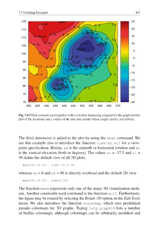
Fig. 7.6 Filled contours used together with a colorbar displaying a legend for the graph and the
plot of the locations and z-values of the true data points (black empty circles, text labels).
The third dimension is added to the plot by using the mesh command. We
use this example also to introduce the function view(az,el) for a view-
point specifi cation. Herein, az is the azimuth or horizontal rotation and el
is the vertical elevation (both in degrees). The values az = -37.5 and el =

30 define the default view of all 3D plots,
mesh(XI,YI,ZI), view(-37.5,30)
whereas az = 0 and el = 90 is directly overhead and the default 2D view

mesh(XI,YI,ZI), view(0,90)

The function mesh represents only one of the many 3D visualization meth-
ods. Another commonly used command is the function surf. Furthermore,

the figure may be rotated by selecting the Rotate 3D option on the Edit Tools
menu. We also introduce the function colormap, which uses predefi ned
pseudo colormaps for 3D graphs. Typing help graph3d lists a number
of builtin colormaps, although colormaps can be arbitrarily modifi ed and