Page 169 - MATLAB Recipes for Earth Sciences

164 7 Spatial Data

square or the root of distance may also be used instead of weighing the z val-

ues by the inverse of distance. The fitting of 3D splines to the control points
provides another method for computing the grid points that is commonly
used in the earth sciences. Most routines used in surface estimation involve

cubic polynomial splines, i.e., a third-degree 3D polynomial is fitted to at

least six adjacent control points. The final surface consists of a composite
of pieces of these splines. MATLAB also provides interpolation with bihar-
monic splines generating very smooth surfaces (Sandwell, 1987).

7.7 Gridding Example

MATLAB provides a biharmonic spline interpolation since its very begin-
nings. This interpolation method was developed by Sandwell (1987). This

specific gridding method produces smooth surfaces that are particularly
suited for noisy data sets with irregular distribution of control points. As an
example we use synthetic xyz data representing the vertical distance of an
imaginary surface of a stratigraphic horizon from a reference surface. This
lithologic unit was displaced by a normal fault. The foot wall of the fault
shows more or less horizontal strata, whereas the hanging wall is charac-
terized by the development of two large sedimentary basins. The xyz data
are irregularly distributed and have to be interpolated onto a regular grid.
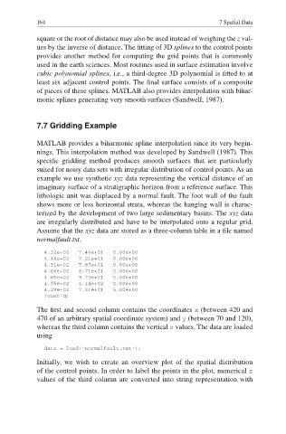
Assume that the xyz data are stored as a three-column table in a fi le named
normalfault.txt.

4.32e+02 7.46e+01 0.00e+00
4.46e+02 7.21e+01 0.00e+00
4.51e+02 7.87e+01 0.00e+00
4.66e+02 8.71e+01 0.00e+00
4.65e+02 9.73e+01 0.00e+00
4.55e+02 1.14e+02 0.00e+00
4.29e+02 7.31e+01 5.00e+00
(cont’d)

The first and second column contains the coordinates x (between 420 and
470 of an arbitrary spatial coordinate system) and y (between 70 and 120),
whereas the third column contains the vertical z values. The data are loaded
using
data = load('normalfault.txt');

Initially, we wish to create an overview plot of the spatial distribution
of the control points. In order to label the points in the plot, numerical z
values of the third column are converted into string representation with