Page 232 - MATLAB Recipes for Earth Sciences

228 9 Multivariate Statistics

Separated Signals − PCA Separated Signals − ICA
4 4
2 2
0 0
s PCA1 −2 s ICA1 −2
−4 −4
0 1000 2000 3000 4000 0 1000 2000 3000 4000
a b
2 4
2
0
s PCA2 −2 s ICA2 −2
0
−4 −4
0 1000 2000 3000 4000 0 1000 2000 3000 4000
c d
2 4
s PCA3 1 0 s ICA3 2

−1 0
−2 −2
0 1000 2000 3000 4000 0 1000 2000 3000 4000
e f
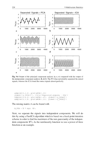
Fig. 9.6 Output of the principal component analysis (a, c, e) compared with the output of
the independent component analysis (b, d, f). The PCA has not reliably separated the mixed
signals, whereas the ICA found the source signals almost perfectly.

subplot(3,2,1), plot(sPCA(:,1))
ylabel('s_{PCA1}'), title('Separated signals - PCA')
subplot(3,2,3), plot(sPCA(:,2)), ylabel('s_{PCA2}')
subplot(3,2,5), plot(sPCA(:,3)), ylabel('s_{PCA3}')
The mixing matrix A can be found with

A_PCA = E * sqrt (D);

Next, we separate the signals into independent components. We will do
this by using a FastICA algorithm which is based on a fi xed-point iteration

scheme in order to find the maximum of the non-gaussianity of the indepen-
T
dent components W x. As the nonlinearity function we use a power of three
function as an example.