Page 227 - MATLAB Recipes for Earth Sciences

9.3 Cluster Analysis 223

The second step in performing a cluster analysis is to rank the groups by
their similarity and build a hierarchical tree visualized as a dendrogram.

Defining groups of objects with significant similarity and separating clusters
depends on the internal similarity and the difference between the groups.
Most clustering algorithms simply link the two objects with highest simi-
larity. In the following steps, the most similar pairs of objects or clusters
are linked iteratively. The difference between groups of objects forming a
cluster is described in different ways depending on the type of data and ap-
plication.

1. K-means clustering – Here, the Euclidean distance between the multi-
variate means of the K clusters are used as a measure for the difference
between the groups of objects. This distance is used if the data suggest
that there is a true mean value surrounded by random noise.

2. K-nearest-neighbors clustering – Alternatively, the Euclidean distance of
the nearest neighbors is used as such a measure. This is used if there is
a natural heterogeneity in the data set that is not attributed to random
noise.

It is important to evaluate the data properties prior to the application of a
clustering algorithm. Firstly, one should consider the absolute values of the
variables. For example, a geochemical sample of volcanic ash might show
SiO contents of around 77% and Na O contents of 3.5%, although the Na O
2 2 2
content is believed to be of great importance. In this case, the data need to
be transformed to zero means ( mean centering). Differences in the vari-
ances and in the means are corrected by autoscaling, i.e., the data are stan-
dardized to zero means and variances that equal one. Artifacts arising from

closed data, such as artificial negative correlations, are avoided by using
Aitchison·s log-ratio transformation (Aitchison 1984, 1986). This ensures
data independence and avoids the constant sum normalization constraints.
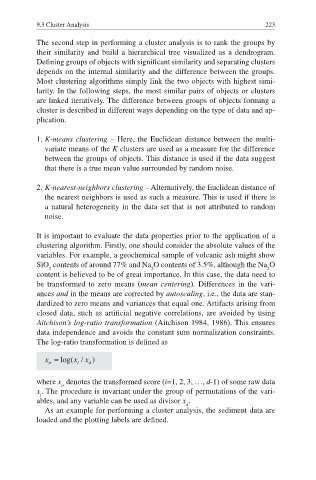
The log-ratio transformation is defi ned as

where x denotes the transformed score (i=1, 2, 3, …, d-1) of some raw data
tr
x . The procedure is invariant under the group of permutations of the vari-
i
ables, and any variable can be used as divisor x .
d
As an example for performing a cluster analysis, the sediment data are
loaded and the plotting labels are defi ned.