Page 225 - MATLAB Recipes for Earth Sciences

9.3 Cluster Analysis 221

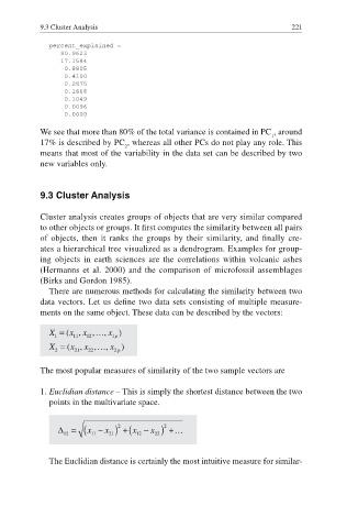
percent_explained =
80.9623
17.1584
0.8805
0.4100
0.2875
0.1868
0.1049
0.0096
0.0000
We see that more than 80% of the total variance is contained in PC , around
1
17% is described by PC , whereas all other PCs do not play any role. This
2
means that most of the variability in the data set can be described by two
new variables only.

9.3 Cluster Analysis

Cluster analysis creates groups of objects that are very similar compared

to other objects or groups. It first computes the similarity between all pairs
of objects, then it ranks the groups by their similarity, and fi nally cre-
ates a hierarchical tree visualized as a dendrogram. Examples for group-
ing objects in earth sciences are the correlations within volcanic ashes
(Hermanns et al. 2000) and the comparison of microfossil assemblages
(Birks and Gordon 1985).
There are numerous methods for calculating the similarity between two
data vectors. Let us define two data sets consisting of multiple measure-

ments on the same object. These data can be described by the vectors:

The most popular measures of similarity of the two sample vectors are

1. Euclidian distance – This is simply the shortest distance between the two
points in the multivariate space.

The Euclidian distance is certainly the most intuitive measure for similar-