Page 224 - MATLAB Recipes for Earth Sciences

220 9 Multivariate Statistics

0.6
qtz
0.4
amp ksp
Second principal component scores −0.2 0 pyr sph
cla
0.2
pla

−0.4
gal flu
−0.6

−0.8
−0.6 −0.4 −0.2 0 0.2 0.4 0.6 0.8
First principal component scores

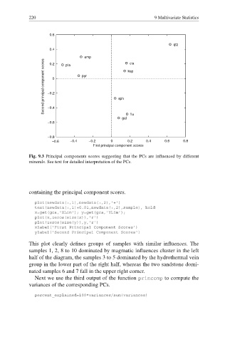
Fig. 9.3 Principal components scores suggesting that the PCs are influenced by different

minerals. See text for detailed interpretation of the PCs.

containing the principal component scores.

plot(newdata(:,1),newdata(:,2),'+')
text(newdata(:,1)+0.01,newdata(:,2),sample), hold
x=get(gca,'XLim'); y=get(gca,'YLim');
plot(x,zeros(size(x)),'r')
plot(zeros(size(y)),y,'r')
xlabel('First Principal Component Scores')
ylabel('Second Principal Component Scores')

This plot clearly defines groups of samples with similar infl uences. The
samples 1, 2, 8 to 10 dominated by magmatic influences cluster in the left

half of the diagram, the samples 3 to 5 dominated by the hydrothermal vein
group in the lower part of the right half, whereas the two sandstone domi-
nated samples 6 and 7 fall in the upper right corner.
Next we use the third output of the function princomp to compute the
variances of the corresponding PCs.

percent_explained=100*variances/sum(variances)