Page 166 - Machine Learning for Subsurface Characterization

140 Machine learning for subsurface characterization

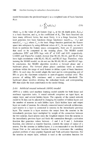
model formulates the predicted target ^ y as a weighted sum of basis function
B(x):
p
X

^ y ¼ α q B q x qi (5.9)
i
q¼1
where x qi is the value of qth feature (log) x q at the ith depth point, B q (x qi )
is a basis function, and α q is the coefficient of B q . The basis function can
have many different forms, but most likely, it is a hinge function. Each
knot generates two basis functions (hinge functions): max(0,x qi C q ) and
max(0,C q x qi ), where C q is the knot. Hinge function partitions the feature
space into subspaces by using different values of C q . In our study, we use 10
knots to partition the feature space; consequently, there are 21 parameters
that need to be computed in the training phase. The MARS model
2
synthesizes DTC and DTS logs with R of 0.85 and 0.83, respectively.
LASSO and ElasticNet models showed that RLA0, RLA4, and RLA5 logs
have high correlations with RLA1, RLA2, and RLA3 logs. Therefore, when
training the MARS model, we do not use the RLA0, RLA4, and RLA5 logs.
In conclusion, the MARS algorithm involves a forward phase and a
backward phase. The forward phase places candidate knots at random
positions within the range of each feature to define a pair of basis functions
(BFs). At each step, the model adapts the knot and its corresponding pair of
BFs to give the maximum reduction in sum-of-squares residual error. This
process of adding BFs continues until a user-defined threshold. The
backward phase involves deleting the redundant knots and corresponding
BFs that made the least contribution to the model fitting.

2.4.6 Artificial neural network (ANN) model
ANN is a widely used machine learning model suitable for both linear and
nonlinear regression tasks. A neural network comprises an input layer, an
output layer, and several hidden layers. The capacity of the neural network
model to fit data can be adjusted by changing the number of hidden layers and
the number of neurons in each hidden layer. Each hidden layer and output
layer are made of neurons. In a densely connected neural network architecture,
each neuron in a layer is connected to neurons in the immediately previous
layer. The neuron in a layer receives the output from the neurons in the
immediately previous layer multiplied by weight of the connection between
the two neurons. Each neuron sums the weighted outputs from the neurons in
the immediately previous layer and feeds the summation through a activation
function that generates values between 1and1or0and1. Activation
function, also referred as transfer function, controls the nature of output of a
neuron. For the neurons in hidden layers, it is recommended to use Rectified
Linear Unit as the activation function because it overcomes the vanishing
gradient problem of once popular Sigmoid and Tanh activation functions. For
the neurons in output layer, softmax is used as the activation function for