Page 111 - Macromolecular Crystallography

100 MACROMOLECULAR CRYS TALLOGRAPHY

In this article, we will restrict ourselves to the case maximum for the true orientation. In its real-space
of finding the orientation and position of a known formulation, it consists of the convolution of the
model in another unit cell, to help solve the molec- experimental Patterson function with the computed
ular structure contained in this unit cell (Fig. 7.2). Patterson of the model in every possible orienta-
Traditionally, this six-dimensional (6D) search (three tion. If restricted to the molecular volume, the use
orientation angles and three translations are to be of Patterson functions allows the superposition of
found) is divided into two separate and consecutive intramolecular vectors, which are independent of
3D search problems. relative translations between the model and the tar-
The first one consists of finding the orientation of get. In its reciprocal-space formulation (Rossmann
the model through the so-called rotation function, and Blow, 1962), it was demonstrated that the max-
which is defined in such a way that it should be imum of this function is indeed the expected solu-
tion. Later on, the formula was rearranged using
the plane-wave expansion and spherical harmon-
ics so as to use the powerful technique of Fast
Fourier Techniques (FFT) (Crowther, 1972), whose
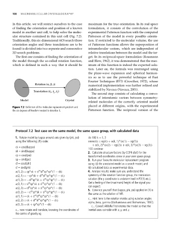
Rotation (α, β, γ) numerical implementation was further refined and
stabilized by Navaza (Navaza, 2001).
Translation (t x , t y ,t z )
The second step consists of calculating a convo-
lution of interatomic vectors between symmetry-
Model Crystal
related molecules of the correctly oriented model
Figure 7.2 Definition of the molecular replacement problem and placed at different origins, with the experimental
the six degrees of freedom needed to describe it. Patterson function. The reciprocal version of the

Protocol 7.2 Test case on the same model, the same space group, with calculated data

1. Rotate model by kappa around axis given by (phi, psi) do 100 k = 1, 3
∗
using the following jiffy code: xnew(k) = xg(k) + a(k, 1) (x(1) − xg(1))
+ a(k, 2) (x(2) − xg(2)) + a(k, 3) (x(3) − xg(3))
∗
∗
ck = cosd(kappa)
100 continue
sk = sind(kappa)
2. Calculate structure factors (by CCP4 sfall) for the
cp = cosd(psi) transformed coordinates xnew in your own space group.
sp = sind(psi) 3. Run your favourite molecular replacement program
cf = cosd(phi) using: (i) the unrotated model as a search model; and
sf = sind(phi) (ii) calculated data as experimental data.
∗ ∗
∗
∗
∗
a(1, 2) = cp sk + cf sf sp sp (1 − ck) 4. Analyse results: make sure you understand the
∗ ∗
∗
∗
∗
a(2, 1) =−cp sk + cf sf sp sp (1 − ck) symmetry of the rotation function group, the translation
∗
∗
∗
∗
∗
a(1, 3) =−sf sp sk + cf cp sp (1 − ck) solution (the y coordinate is undetermined in P2(1) etc.).
Get a feeling of the (maximum) height of the signal you
∗
∗
∗
∗
∗
a(3, 1) = sf sp sk + cf cp sp (1 − ck)
can expect.
∗
∗
∗
∗
∗
a(2, 3) = cf sp sk + sf cp sp (1 − ck)
5. Convince yourself that (kappa, phi, psi) applied in (1) is
∗
∗
∗
∗
∗
a(3, 2) =−cf sp sk + sf cp sp (1 − ck)
the same as the solution of MR.
∗ ∗
∗
∗
a(1, 1) = ck + cf cf sp sp (1 − ck)
c... Hint: here is the rotation matrix using eulerian angles
∗
∗ ∗
∗
a(2, 2) = ck + sf sf sp sp (1 − ck)
alpha, beta, gamma (Urzhumtseva and Urzhumtsev, 1997).
∗
∗
a(3, 3) = ck + cp cp (1 − ck)
c... Caveat:AMoRe first rotates the model so that the
c... now rotate and translate, knowing the coordinates of inertial axes coincide with x, y, and z.
the centre of gravity xg