Page 112 - Macromolecular Crystallography

MOLECULAR REPLACEMENT TECHNIQUES 101

calculation lends itself particularly well to Fourier • type of score used as an indicator of the quality of
(Crowther and Blow, 1967) and FFT techniques and the agreement.
is, in general, very rapid.
Usually, the top peaks of the translation search This is reflected in the following input parameters:
are then submitted to a low resolution quick
rigid-body refinement, for which quick algorithms • quality of the X-ray data (see Protocol 7.1)
have been devised (Huber and Schneider, 1985; • quality of the model(s), e.g. poly-Ala versus full
Navaza and Saludjian, 1997).The resolution is usu- model (see below, structural diversity)
ally taken to be 12–4 Ångstroms or so; if one wants • number of molecules per asymmetric unit
to use the low resolution terms, one should use • target functions.
a solvent effect correction technique (Fokine and
Urzhumtsev, 2002). While the first point was addressed directly in
The following issues are crucial for the success of Protocol 7.1, we will address the other points suc-
the method: cessively in the next paragraphs.
Before executing the real MR protocol, we
• completeness and quality of the data strongly recommend running a test case. Under-
• accuracy of the model(s) standing the conventions of the rotation func-
• completeness of the modelling of the unit cell tion will be greatly facilitated by reading a recent

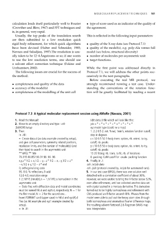
Protocol 7.3 A typical molecular replacement session using AMoRe (Navaza, 2001)
1. Read the Manual! Edit dato.i3 file which will look like this:
∗
∗
∗
∗
∗
∗
2. Move to an empty directory and type : csh job + + + + + + + + + ∗
∗
∗
$AMORE/setup xyz model type (could ne a map)
3. Then: 1. 2 2 0.5 2. rot: %rad, 1min’s, rotation function cutoff,
In ./d/: step in degrees
– Create data.d (as data.example created by setup), c-c 50 0.5 50 1-body trans: option, nb. orient. to try,
and give cell parameters, symmetry related positions, cutoff, nb. peaks
resolution limits, and the number of molecule(s) (and p-t 10 0.5 50 n-body trans: option, nb. orient. to try,
their type) to search in the asymmetric unit cutoff, nb. peaks
6PGL Title 10 20 fitting: nb. trans. to fit, nb. of iterations
∗∗ ∗∗
70.315 80.852 90.31 90. 90. 90. 0. packing: CoM cutoff for -crude- packing function
x,y,z 1/2 + x,1/2 − y,−z 1/2 − x,−y,1/2 + z ∗ 4. Finally, in ./:
∗
∗
∗
−x,1/2 + y,1/2 − z end csh ./e/job dato
0; orthogonalizing code csh ./job (protocol created by ./e/job for automated runs).
95. 0.0; % reflections, B-add 5. In our test case (6PGL), there was one solution well
12.0 4.0; resolution range detached with a correlation coefficient of about 30%.
1 2; NTYP, (nmol(n),n = 1,NTYP); a homodimer in the However, we were unable to bring the R-factor below 52%,
asymmetric unit even after refinement, until we collected another data set
– Data files with diffraction data and model coordinates with crystal soaked in a mercury derivative. This derivative
must be named hkl.d and xyzN.d, respectively; N = 1 for turned out to be highly isomorphous and refinement with
the first model, N = 2 for the second one... CNS produced an R-factor around 48%. Phases from the
Insert FORMAT card (upper case) in hkl.d and xyz{#}.d model were able to pull out the heavy atom sites through
files (as hkl.example and xyz1.example created by both isomorphous and anomalous Fourier difference maps.
setup). The resulting solvent-flattened 2.8 Ångstrom SIRAS map
– In ./i/: was interpretable.