Page 142 - Macromolecular Crystallography

APPLICATION OF DIRECT METHODS 131

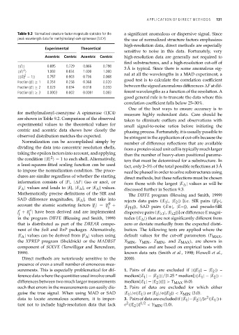
Table 9.2 Normalized structure-factor magnitude statistics for the a significant anomalous or dispersive signal. Since
peak-wavelength data for methylmalonyl-coA epimerase (1JC4) the use of normalized structure factors emphasizes
high-resolution data, direct methods are especially
Experimental Theoretical
sensitive to noise in this data. Fortunately, very
Acentric Centric Acentric Centric high-resolution data are generally not required to
find substructures, and a high-resolution cut-off of
|E| 0.885 0.729 0.866 0.798
2 3 Å is typical. Since there is some anomalous sig-
|E| 1.002 0.834 1.000 1.000
2 nal at all the wavelengths in a MAD experiment, a
||E| − 1| 0.757 0.903 0.736 0.968
good test is to calculate the correlation coefficient
Fraction |E|≥ 1 0.351 0.258 0.368 0.320
between the signed anomalous differences F at dif-
Fraction |E|≥ 2 0.023 0.034 0.018 0.050
Fraction |E|≥ 3 0.0003 0.002 0.0001 0.003 ferent wavelengths as a function of the resolution. A
good general rule is to truncate the data where this
correlation coefficient falls below 25–30%.
One of the best ways to ensure accuracy is to
for methylmalonyl-coenzyme A epimerase (1JC4) measure highly redundant data. Care should be
are shown in Table 9.2. Comparison of the observed taken to eliminate outliers and observations with
experimental values to the theoretical values for small signal-to-noise ratios before initiating the
centric and acentric data shows how closely the phasing process. Fortunately, it is usually possible to
observed distribution matches the expected. be stringent in the application of cut-offs because the
Normalization can be accomplished simply by number of difference reflections that are available
dividing the data into concentric resolution shells, from a protein-sized unit cell is typically much larger
taking the epsilon factors into account, and applying than the number of heavy-atom positional parame-
2
the condition |E| = 1 to each shell. Alternatively, ters that must be determined for a substructure. In
a least-squares-fitted scaling function can be used fact, only 2–3% of the total possible reflections at 3 Å
to impose the normalization condition. The proce- need be phased in order to solve substructures using
dures are similar regardless of whether the starting direct methods, but these reflections must be chosen
information consists of |F|, | F| (iso or ano), or from those with the largest |E | values as will be
|F A | values and leads to |E|, |E |,or |E A | values.
discussed further in Section 9.3.
Mathematically precise definitions of the SIR and
The DIFFE program (Blessing and Smith, 1999)
SAD difference magnitudes, |E |, that take into rejects data pairs (|E 1 |, |E 2 |) [i.e. SIR pairs (|E P |,
0
account the atomic scattering factors |f j |=|f +
j |E PH |), SAD pairs (|E+|, |E−|), and pseudo-SIR

f + if | have been derived and are implemented dispersive pairs (|E λ1 |, |E λ2 |)] or difference E magni-
j j
in the program DIFFE (Blessing and Smith, 1999) tudes (|E |) that are not significantly different from
that is distributed as part of the DREAR compo- zero or deviate markedly from the expected distri-
nent of the SnB and BnP packages. Alternatively, bution. The following tests are applied where the
|E A | values can be derived from |F A | values using default values for the cut-off parameters (T MAX ,
the XPREP program (Sheldrick) or the MADBST X MIN , Y MIN , Z MIN , and Z MAX ), are shown in
component of SOLVE (Terwilliger and Berendzen, parentheses and are based on empirical tests with
1999). known data sets (Smith et al., 1998; Howell et al.,
Direct methods are notoriously sensitive to the 2000).
presence of even a small number of erroneous mea-
surements. This is especially problematical for dif- 1. Pairs of data are excluded if |(|E 1 |−|E 2 |) –
ference data where the quantities used involve small median(|E 1 |−|E 2 |)|/{1.25 * median[|(|E 1 |−|E 2 |) –
differences between two much larger measurements median(|E 1 |−|E 2 |)|]} > T MAX (6.0).
such that errors in the measurements can easily dis- 2. Pairs of data are excluded for which either
guise the true signal. When using MAD or SAD |E 1 |/σ(|E 1 |) or |E 2 |/σ(|E 2 |)< X MIN (3.0).
2
data to locate anomalous scatterers, it is impor- 3. Pairsofdataareexcludedif||E 1 |−|E 2 ||/[σ (|E 1 |)+
2
tant not to include high-resolution data that lack σ (|E 2 |)] 1/2 < Y MIN (1.0).