Page 173 - Materials Science and Engineering An Introduction

5.4 Fick’s Second Law—Nonsteady-State Diffusion • 145

EXAMPLE PROBLEM 5.1

Diffusion Flux Computation
A plate of iron is exposed to a carburizing (carbon-rich) atmosphere on one side and a decar-
burizing (carbon-deficient) atmosphere on the other side at 700 C (1300 F). If a condition of
steady state is achieved, calculate the diffusion flux of carbon through the plate if the concen-
3
2
trations of carbon at positions of 5 and 10 mm (5 10 and 10 m) beneath the carburizing
2
3
surface are 1.2 and 0.8 kg/m , respectively. Assume a diffusion coefficient of 3 10 11 m /s at
this temperature.
Solution
Fick’s first law, Equation 5.2, is used to determine the diffusion flux. Substitution of the values
just given into this expression yields

(1.2 - 0.8) kg/m 3
C A - C B -11 2
J = -D = -(3 * 10 m /s) -3 -2
x A - x B (5 * 10 - 10 ) m
2
-9
= 2.4 * 10 kg/m # s
5.4 FICK’S SECOND LAW—NONSTEADY-STATE
DIFFUSION
Most practical diffusion situations are nonsteady-state ones—that is, the diffusion flux
and the concentration gradient at some particular point in a solid vary with time, with
a net accumulation or depletion of the diffusing species resulting. This is illustrated in
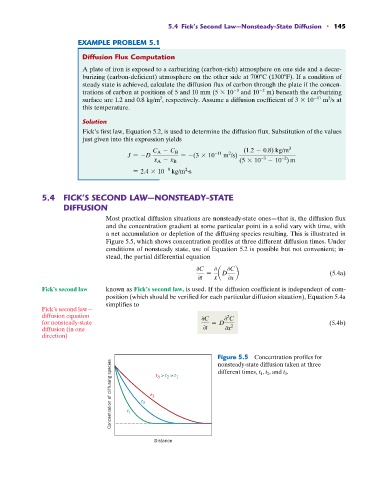
Figure 5.5, which shows concentration profiles at three different diffusion times. Under
conditions of nonsteady state, use of Equation 5.2 is possible but not convenient; in-
stead, the partial differential equation

0C 0 0C
= aD b (5.4a)
0t x 0x
Fick’s second law known as Fick’s second law, is used. If the diffusion coefficient is independent of com-
position (which should be verified for each particular diffusion situation), Equation 5.4a
simplifies to
Fick’s second law—
diffusion equation 2
for nonsteady-state 0C = D 0 C (5.4b)
diffusion (in one 0t 0x 2
direction)

Figure 5.5 Concentration profiles for
Concentration of diffusing species t 1 t 2 t 3 3 2 1
nonsteady-state diffusion taken at three
different times, t 1 , t 2 , and t 3 .
t > t > t

Distance