Page 286 - Mathematical Models and Algorithms for Power System Optimization

278 Chapter 7

2 3
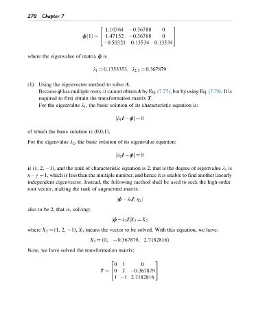
1:10364 0:36788 0
ϕ 1ðÞ ¼ 4 1:47152 0:36788 0 5
0:50321 0:13534 0:13534

where the eigenvalue of matrix ϕ is

λ 1 ¼ 0:1353353, λ 2,3 ¼ 0:367879

(1) Using the eigenvector method to solve A.
Because ϕ has multiple roots, it cannot obtain A by Eq. (7.77), but by using Eq. (7.78).Itis
required to first obtain the transformation matrix T.
For the eigenvalue λ 1 , the basic solution of its characteristic equation is:

j λ 1 I ϕj ¼ 0

of which the basic solution is (0,0,1).
For the eigenvalue λ 2 , the basic solution of its eigenvalue equation:

j λ 2 I ϕj ¼ 0

is (1, 2, 1), and the rank of characteristic equation is 2, that is the degree of eigenvalue λ 1 is
n – γ ¼1, which is less than the multiple number, and hence it is unable to find another linearly
independent eigenvector. Instead, the following method shall be used to seek the high-order
root vector, making the rank of augmented matrix:

½ ϕ λ 3 Ij η Š
2
also to be 2, that is, solving:

j ϕ λ 3 IjX 3 ¼ X 2

where X 2 ¼(1, 2, 1), X 3 means the vector to be solved. With this equation, we have:
X 3 ¼ 0, 0:367879, 2:7182816ð Þ

Now, we have solved the transformation matrix:

2 3
01 0
T ¼ 02 0:367879 5
4
1 12:7182816