Page 284 - Mathematical Models and Algorithms for Power System Optimization

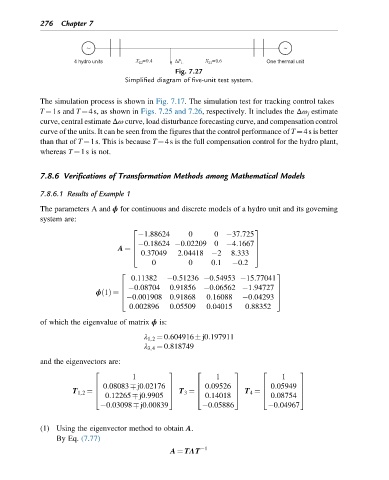
276 Chapter 7

4 hydro units One thermal unit
Fig. 7.27
Simplified diagram of five-unit test system.

The simulation process is shown in Fig. 7.17. The simulation test for tracking control takes
T¼1s and T¼4s, as shown in Figs. 7.25 and 7.26, respectively. It includes the Δω j estimate
curve, central estimate Δω curve, load disturbance forecasting curve, and compensation control
curve of the units. It can be seen from the figures that the control performance of T¼4s is better
than that of T¼1s. This is because T¼4s is the full compensation control for the hydro plant,
whereas T¼1s is not.

7.8.6 Verifications of Transformation Methods among Mathematical Models

7.8.6.1 Results of Example 1

The parameters A and ϕ for continuous and discrete models of a hydro unit and its governing
system are:

2 3
1:88624 0 0 37:725
0:18624 0:02209 0 4:1667
6 7
A ¼ 6 7
4 0:37049 2:04418 2 8:333 5
0 0 0:1 0:2
2 3
0:11382 0:51236 0:54953 15:77041
0:08704 0:91856 0:06562 1:94727
6 7
ϕ 1ðÞ ¼ 6 7
0:001908 0:91868 0:16088 0:04293
4 5
0:002896 0:05509 0:04015 0:88352
of which the eigenvalue of matrix ϕ is:
λ 1,2 ¼ 0:604916 j0:197911
λ 3,4 ¼ 0:818749
and the eigenvectors are:
2 3 2 3 2 3
1 1 1
6 0:08083 j0:02176 7 6 0:09526 7 6 0:05949 7
T 1,2 ¼ 6 7 T 3 ¼ 6 7 T 4 ¼ 6 7
4 0:12265 j0:9905 5 4 0:14018 5 4 0:08754 5
0:03098 j0:00839 0:05886 0:04967

(1) Using the eigenvector method to obtain A.
By Eq. (7.77)

A ¼ TΛT 1