Page 285 - Mathematical Models and Algorithms for Power System Optimization

Optimization Method for Load Frequency Feed Forward Control 277

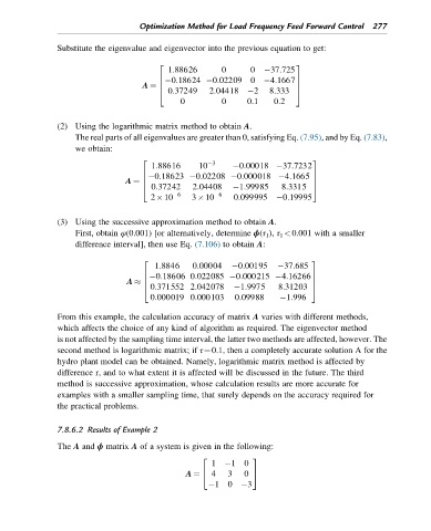
Substitute the eigenvalue and eigenvector into the previous equation to get:

2 3
1:88626 0 0 37:725
0:18624 0:02209 0 4:1667
6 7
A ¼ 6 7
4 0:37249 2:04418 2 8:333 5
0 0 0:1 0:2

(2) Using the logarithmic matrix method to obtain A.
The real parts of all eigenvalues are greater than 0, satisfying Eq. (7.95), and by Eq. (7.83),
we obtain:
2 3 3
1:88616 10 0:00018 37:7232
6 0:18623 0:02208 0:000018 4:1665 7
A ¼ 6 7
4 0:37242 2:04408 1:99985 8:3315 5
2 10 6 3 10 6 0:099995 0:19995

(3) Using the successive approximation method to obtain A.
First, obtain φ(0.001) [or alternatively, determine ϕ(τ 1 ), τ 1 <0.001 with a smaller
difference interval], then use Eq. (7.106) to obtain A:

2 3
1:8846 0:00004 0:00195 37:685
6 0:18606 0:022085 0:000215 4:16266 7
A 6 7
4 0:371552 2:042078 1:9975 8:31203 5
0:000019 0:000103 0:09988 1:996

From this example, the calculation accuracy of matrix A varies with different methods,
which affects the choice of any kind of algorithm as required. The eigenvector method
is not affected by the sampling time interval, the latter two methods are affected, however. The
second method is logarithmic matrix; if τ¼0.1, then a completely accurate solution A for the
hydro plant model can be obtained. Namely, logarithmic matrix method is affected by
difference r, and to what extent it is affected will be discussed in the future. The third
method is successive approximation, whose calculation results are more accurate for
examples with a smaller sampling time, that surely depends on the accuracy required for
the practical problems.

7.8.6.2 Results of Example 2
The A and ϕ matrix A of a system is given in the following:

2 3
1 10
A ¼ 4 4 3 0 5
10 3