Page 39 - Mathematical Models and Algorithms for Power System Optimization

Daily Economic Dispatch Optimization With Pumped Storage Plant 29

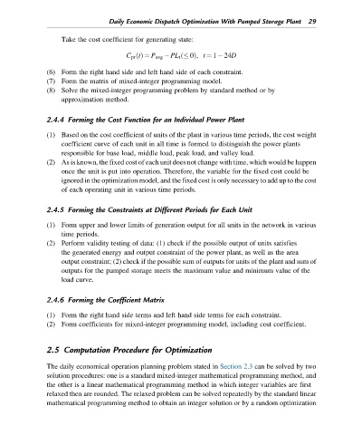
Take the cost coefficient for generating state:

C pr tðÞ ¼ P avg PL t 0ð Þ, t ¼ 1 24D

(6) Form the right hand side and left hand side of each constraint.
(7) Form the matrix of mixed-integer programming model.
(8) Solve the mixed-integer programming problem by standard method or by
approximation method.

2.4.4 Forming the Cost Function for an Individual Power Plant

(1) Based on the cost coefficient of units of the plant in various time periods, the cost weight
coefficient curve of each unit in all time is formed to distinguish the power plants
responsible for base load, middle load, peak load, and valley load.
(2) As is known, the fixed cost of each unit does not change with time, which would be happen
once the unit is put into operation. Therefore, the variable for the fixed cost could be
ignored in the optimization model, and the fixed cost is only necessary to add up to the cost
of each operating unit in various time periods.

2.4.5 Forming the Constraints at Different Periods for Each Unit
(1) Form upper and lower limits of generation output for all units in the network in various
time periods.
(2) Perform validity testing of data: (1) check if the possible output of units satisfies
the generated energy and output constraint of the power plant, as well as the area
output constraint; (2) check if the possible sum of outputs for units of the plant and sum of
outputs for the pumped storage meets the maximum value and minimum value of the
load curve.

2.4.6 Forming the Coefficient Matrix

(1) Form the right hand side terms and left hand side terms for each constraint.
(2) Form coefficients for mixed-integer programming model, including cost coefficient.

2.5 Computation Procedure for Optimization

The daily economical operation planning problem stated in Section 2.3 can be solved by two
solution procedures: one is a standard mixed-integer mathematical programming method, and
the other is a linear mathematical programming method in which integer variables are first
relaxed then are rounded. The relaxed problem can be solved repeatedly by the standard linear
mathematical programming method to obtain an integer solution or by a random optimization