Page 44 - Mathematical Models and Algorithms for Power System Optimization

34 Chapter 2

power plant (two units), and one pumped storage plant (one unit), where two calculation time
periods (i, j) are considered. According to the proposed mathematical model, the variables of
the two thermal units in two time periods are X i1 , X i2 , X j1 , X j2 ; the generating and pumping
variables of the pumped storage unit are x g1 , x g2 and y p1 , y p2 .

The number of constraints the number of time period (load)+the number of power
plants the number of time periods (power plant generated output)+the number of power
plants (power plant generated energy)+the number of areas the number of time periods (area
generated output)+the number of time periods (pumping output)+1 (water balancing)¼2
+1 2+1+1 2+2+1¼10.
The number of continuous variables¼the number of units the number of time
periods¼3 2¼6, the number of integer variables¼the number of time periods¼2, and total
number of variables¼8.
Thus, it can be seen that the number of constraints in the model is irrelevant to the number
of units, and there should be at least five units to make the model solvable (because the
number of variables has to be greater than that of constraints in the LP calculation). Generally,
an actual system can meet this requirement. Due to space limitations, the objective and
constraint function expressions for a small-scale test system with only two units are shown
as follows.

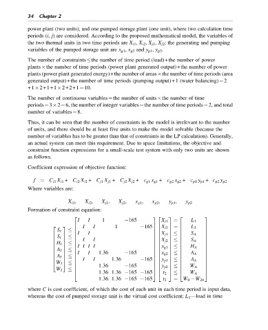
Coefficient expression of objective function:

f ¼ C i1 X i1 + C i2 X i2 + C j1 X j1 + C j2 X j2 + c g1 x g1 + c g2 x g2 + c p1 y p1 + c p2 y p2
Where variables are:

X i1 , X i2 , X j1 , X j2 , x g1 , x g2 , y p1 , y p2
Formation of constraint equation:

2 32 3 2 3
I I 1 165 X i1 ¼ L 1
I I 1 165
6 76 7 ¼ 6 7
2 3 X i2 L 2
S I 6 76 7 6 7
I I
6 76 X j1 7 6 S A 7
S I
6 7 6 76 7 6 7
6 7 6 I I 76 X j2 7 6 S A 7
H I
6 7 6 76 7 6 7
6 7 6 I III 76 x g1 7 6 H A 7
A I
6 7 6 76 7 6 7
6 7 6 I I 1:36 165 76 x g2 7 6 A A 7
A I
6 7 6 76 7 6 7
6 7 6 I I 1:36 165 76 y p1 7 6 A A 7
W I
4 5 6 76 7 6 7
6 1:36 165 76 7 6 W A 7
W I 6 76 y p2 7 6 7
4 1:36 1:36 165 165 54 t 2 5 4 W A 5
1:36 1:36 165 165 t 2 ¼ W 0 W 24
where C is cost coefficient, of which the cost of each unit in each time period is input data,
whereas the cost of pumped storage unit is the virtual cost coefficient; L 1 —load in time