Page 46 - Mathematical Models and Algorithms for Power System Optimization

36 Chapter 2

Table 2.4 Scale of variables of the practical scale system

(1+30+6+1) 24D+30 930D
The number of constraints<the number of time
periods (load balancing)+the number of power D¼1, 2, 4
plants the number of time periods (power plant
generated output)+the number of power plants
(power plant generated energy)+the number of
areas the number of time periods (area output)+the
number of time periods (pumping reservoir capacity)
+1 (pumping water balance)
100 24D¼2400D
The number of continuous variables¼(total number
of units) the number of time periods
1 24D¼24D
The number of integer variables<the number of time
periods

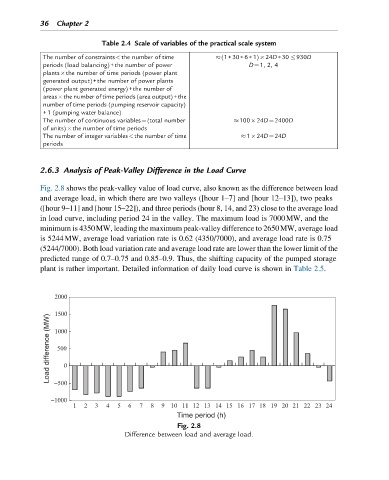
2.6.3 Analysis of Peak-Valley Difference in the Load Curve

Fig. 2.8 shows the peak-valley value of load curve, also known as the difference between load
and average load, in which there are two valleys ([hour 1–7] and [hour 12–13]), two peaks
([hour 9–11] and [hour 15–22]), and three periods (hour 8, 14, and 23) close to the average load
in load curve, including period 24 in the valley. The maximum load is 7000MW, and the
minimum is 4350MW, leading the maximum peak-valley difference to 2650MW, average load
is 5244MW, average load variation rate is 0.62 (4350/7000), and average load rate is 0.75
(5244/7000). Both load variation rate and average load rate are lower than the lower limit of the
predicted range of 0.7–0.75 and 0.85–0.9. Thus, the shifting capacity of the pumped storage
plant is rather important. Detailed information of daily load curve is shown in Table 2.5.

Load difference (MW)

Time period (h)
Fig. 2.8

Difference between load and average load.