Page 54 - Mathematical Models and Algorithms for Power System Optimization

44 Chapter 2

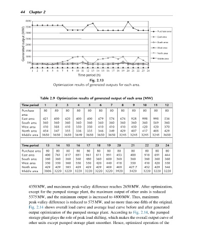
Generated output (MW) Purchase area

East area
South area
West area
North area
Middle area

Time period (h)
Fig. 2.13
Optimization results of generated outputs for each area.

Table 2.9 Optimization results of generated output of each area (MW)
Time period 1 2 3 4 5 6 7 8 9 10 11 12

Purchase 80 80 80 80 80 80 80 80 80 80 80 80
area
East area 421 400 420 400 400 479 576 676 928 998 998 536
South area 360 360 360 360 360 360 360 360 360 360 569 360
West area 410 388 410 350 350 410 410 410 450 420 420 370
North area 454 347 355 336 335 346 349 429 407 417 408 429
Middle area 3650 3650 3650 3649 3650 3650 3650 3245 3245 3245 3245 3650

Time period 13 14 15 16 17 18 19 20 21 22 23 24
Purchase area 80 80 80 80 80 80 80 80 80 80 80 80
East area 400 761 817 881 961 811 991 453 400 918 691 444
South area 360 360 360 360 480 360 600 360 360 360 360 360
West area 350 350 360 350 350 420 440 418 350 410 420 350
North area 429 429 383 429 429 429 469 469 427.7 432 429 346
Middle area 3806 3220 3220 3220 3220 3220 3220 3920 3420 3220 3220 3220

4350MW, and maximum peak-valley difference reaches 2650MW. After optimization,
except for the pumped storage plant, the maximum output of other units is reduced
5375MW, and the minimum output is increased to 4800MW. Thus, maximum
peak-valley difference is reduced to 575MW, and no more than one-fifth of the original.
Fig. 2.14 shows overall load curve and average load curve before and after generated
output optimization of the pumped storage plant. According to Fig. 2.14, the pumped
storage plant plays the role of peak load shifting, which makes the overall output curve of
other units except pumped storage plant smoother. Hence, optimized operation of the