Page 98 - Mathematical Techniques of Fractional Order Systems

86 Mathematical Techniques of Fractional Order Systems

Remark 2: As explained in detail in Casagrande et al. (2017), the introduc-
tion of the auxiliary term is necessary to make the number of unknowns in
a
(3.22) equal to the number of equations. If the poles of Y ðwÞ are fixed, this
Σ
a
result is obtained when the orders of Y ðwÞ and UðsÞ are equal, i.e., the
Σ
a
degree of the denominator of Y ðwÞ coincides with the degree n u of the
Σ
denominator of UðwÞ. The solution is then obtained by equating the coeffi-
r
cients of the equal powers of w at the numerators of the product W ðwÞUðwÞ
ν
a
and of Y U ðwÞ 1 Y ðwÞ 1 Y ðwÞ, respectively. The problem turns out to be
Σ
Σ
linear.
a
Remark 3: If the poles of Y ðwÞ are located far to the left of the imaginary
Σ
axis, this additional term does not alter appreciably the transient dynamics
of the system while it leaves unchanged the input component.
Remark 4: Due to the introduction of the auxiliary term, the order r of
ν
r
W ðwÞ is greater than the order ν of the function Y ðwÞ approximating the
Σ
original system component Y Σ ðwÞ. However, since usually ν{n, the order
r 5 ν 1 n u is still much smaller than n for the canonical inputs (n u # 2 for
steps, ramps and sinusoids).
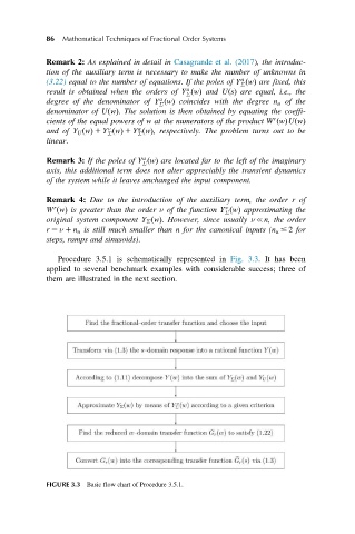
Procedure 3.5.1 is schematically represented in Fig. 3.3. It has been
applied to several benchmark examples with considerable success; three of
them are illustrated in the next section.

FIGURE 3.3 Basic flow chart of Procedure 3.5.1.