Page 102 - Mathematical Techniques of Fractional Order Systems

90 Mathematical Techniques of Fractional Order Systems

0.3
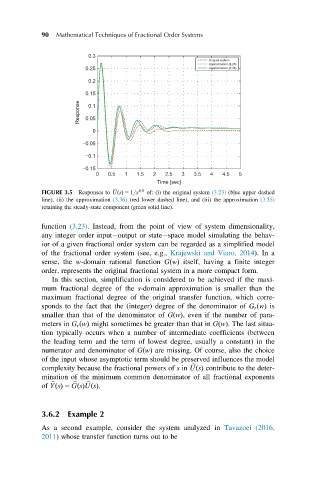
Original system
Approximation (2.26)
0.25 Approximation (2.36)
0.2
0.15
Response 0.05
0.1

0
−0.05
−0.1
−0.15
0 0.5 1 1.5 2 2.5 3 3.5 4 4.5 5
Time [sec]
FIGURE 3.5 Responses to b UðsÞ 5 1=s 0:8 of: (i) the original system (3.23) (blue upper dashed
line), (ii) the approximation (3.36) (red lower dashed line), and (iii) the approximation (3.35)
retaining the steady-state component (green solid line).

function (3.23). Instead, from the point of view of system dimensionality,
any integer order input output or state space model simulating the behav-
ior of a given fractional order system can be regarded as a simplified model
of the fractional order system (see, e.g., Krajewski and Viaro, 2014). In a
sense, the w-domain rational function GðwÞ itself, having a finite integer
order, represents the original fractional system in a more compact form.
In this section, simplification is considered to be achieved if the maxi-
mum fractional degree of the s-domain approximation is smaller than the
maximum fractional degree of the original transfer function, which corre-
sponds to the fact that the (integer) degree of the denominator of G r ðwÞ is
smaller than that of the denominator of GðwÞ, even if the number of para-
meters in G r ðwÞ might sometimes be greater than that in GðwÞ. The last situa-
tion typically occurs when a number of intermediate coefficients (between
the leading term and the term of lowest degree, usually a constant) in the
numerator and denominator of GðwÞ are missing. Of course, also the choice
of the input whose asymptotic term should be preserved influences the model
complexity because the fractional powers of s in UðsÞ contribute to the deter-
b
mination of the minimum common denominator of all fractional exponents
of YðsÞ 5 GðsÞUðsÞ.
b
b
b
3.6.2 Example 2

As a second example, consider the system analyzed in Tavazoei (2016,
2011) whose transfer function turns out to be