Page 104 - Mathematical Techniques of Fractional Order Systems

92 Mathematical Techniques of Fractional Order Systems

The 2nd order optimal Hankel-norm approximation of (3.43) is
B2 2 15:9384z 2 9:9977
Y ðzÞ 5 : ð3:45Þ
Σ
2
z 1 0:3796z 1 0:0511
By adding to (3.45) an auxiliary term with a far-off pole at 2100 (step
(v) of Procedure 3.5.1), and combining the resulting sum with the original
input-dependent component (3.44), the reduced system transfer function in
the z-domain turns out to be

2
B 402:2097z 2 239:7748z 1 102:1383
G r ðzÞ 5 ð3:46Þ
3
2
z 1 100:3796z 1 38:0102z 1 5:1069
and in the s-domain with z 5 s 9=10
402:2097s 1:8 2 239:7748s 0:9 1 102:1383
G r ðsÞ 5 : ð3:47Þ
b
s 2:7 1 100:3796s 1:8 1 38:0102s 0:9 1 5:1069
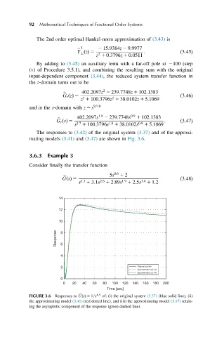
The responses to (3.42) of the original system (3.37) and of the approxi-
mating models (3.41) and (3.47) are shown in Fig. 3.6.

3.6.3 Example 3
Consider finally the transfer function

5s 0:6 1 2
GðsÞ 5 ð3:48Þ
b
s 3:3 1 3:1s 2:6 1 2:89s 1:9 1 2:5s 1:4 1 1:2
14

12

10
Response 8 6

4

2 Original system
Approximation (2.41)
Approximation (2.47)
0
0 20 40 60 80 100 120 140 160 180 200
Time [sec]
FIGURE 3.6 Responses to b UðsÞ 5 1=s 0:9 of: (i) the original system (3.37) (blue solid line), (ii)
the approximating model (3.41) (red dotted line), and (iii) the approximating model (3.47) retain-
ing the asymptotic component of the response (green dashed line).