Page 100 - Mathematical Techniques of Fractional Order Systems

88 Mathematical Techniques of Fractional Order Systems

7
α = 0.1
α = 0.8
α = 0.9
6
5

4
u(t)
3

2

1

0
0 1 2 3 4 5 6
Time
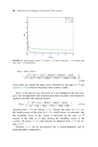
FIGURE 3.4 Input signals of form (3.28) with α 5 0:1 (lower solid line), α 5 0:8 (upper solid
line), and α 5 0:9 (dotted line).

YðwÞ 5 GðwÞ UðwÞ 5
4
8
16
20
12
w 1 9w 1 31w 1 58:01w 1 60:01w 1 16:03 1
5 U
20
4
24
16
w 1 6w 1 48w 1 286w 1 935w 1 1580w 1 888 w 4
8
12
ð3:30Þ
π
whose poles are outside the minor sector delimited by the radii ρe 6 j 10 (see
equation (3.10)) so that the fractional order system is stable.
Since, in this special case, all powers of w are multiples of the same inte-
ger 4, the decomposition and reduction procedures can more conveniently be
applied to the 6th order rational function
3
2
5
4
B z 1 9z 1 31z 1 58:01z 1 60:01z 1 16:03 1
YðzÞ 5 U ; ð3:31Þ
2
3
5
6
z 1 6z 1 48z 1 286z 1 935z 1 1580z 1 888 z
4
4
obtained from (3.30) by setting z 5 w . Clearly, the poles of (3.31) are
the fourth powers of the poles of (3.30), which means, in particular, that
4π
the instability sector in the z-plane is delimited by the radii ρe 6 j 10
π
instead of the radii ρe 6 j 10 that enclose the instability sector in the
w-plane. Of course, (3.31) could directly be obtained from (3.23) by set-
ting z 5 s 4=5 .
Function (3.31) can be decomposed into a system-dependent and an
input-dependent component as