Page 105 - Mathematical Techniques of Fractional Order Systems

Fractional Order System Chapter | 3 93

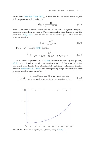
taken from (Xue and Chen, 2007), and assume that the input whose asymp-
totic response must be retained is

10
UðsÞ 5 ð3:49Þ
b
s 0:2 2 0:7s 0:1
which has been chosen, rather arbitrarily, to test the system long-term
response to nondecaying inputs. The corresponding time-domain signal b uðtÞ
is shown in Fig. 3.7. It can be obtained as the step response of a filter with
transfer function
10s 0:9
FðsÞ 5 : ð3:50Þ
b
s 0:1 2 0:7
For w 5 s 0:1 function (3.48) becomes

6
5w 1 2
GðwÞ 5 ; ð3:51Þ
w 1 3:1w 1 2:89w 1 2:5w 1 1:2
33
26
19
14
A 4th order approximation of (3.51) has been obtained by interpolating
(3.51) at s 5 1 and s 5 2 with intersection number 2 (retention of 2 time
moments) according to the multipoint Pade ´ technique via Lanczos’ iteration
method (Gallivan et al., 1996). The corresponding simplified fractional order
transfer function turns out to be
9:6597s 0:3 1 50:106s 0:2 1 56:107s 0:1 1 4:753
G r;PL ðsÞ 5 : ð3:52Þ
b
s 0:4 1 35:5s 0:3 1 161:08s 0:2 1 173:02s 0:1 1 14:037

150

100

50

0
0 10 20 30 40 50 60 70 80 90 100
FIGURE 3.7 Time-domain input signal b uðtÞ corresponding to (3.49).