Page 106 - Mathematical Techniques of Fractional Order Systems

94 Mathematical Techniques of Fractional Order Systems

By applying instead the suggested reduction method based on:
1. the decomposition of YðwÞ 5 GðwÞUðwÞ into a system-dependent
component
X A ðwÞ
Y Σ ðwÞ 5 ð3:53Þ
14
33
26
19
w 1 3:1w 1 2:89w 1 2:5w 1 1:2
and an input-dependent component
X C ðwÞ
Y U ðwÞ 5 ; ð3:54Þ
w 1 w 1 100
2
2. the approximation of (3.53) by means of the same method used to find
(3.52) from (3.48), and
3. the retention of (3.54),
the following approximating fractional order transfer function is obtained
(after substituting s 0:1 for w)
68:447s 0:3 1 357:21s 0:2 1 528:5s 0:1 1 157:17
G r ðsÞ 5 : ð3:55Þ
b
s 0:4 1 3:7838s 0:3 1 103:73s 0:2 1 279:32s 0:1 1 94:3
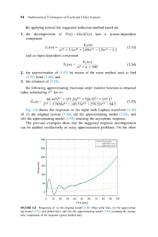
Fig. 3.8 shows the responses to the input with Laplace transform (3.49)
of: (i) the original system (3.48), (ii) the approximating model (3.52), and
(iii) the approximating model (3.55) retaining the asymptotic response.
The previous examples show that the suggested response decomposition
can be applied satisfactorily in many approximation problems. On the other

300
Original system
Approximation (2.52)
Approximation (2.55)
250
200
Response 150

100

50

0

0 10 20 30 40 50 60 70 80 90 100
Time [sec]
FIGURE 3.8 Responses of: (i) the original model (3.48) (blue solid line), (ii) the approximat-
ing model (3.52) (red dotted line), and (iii) the approximating model (3.55) retaining the asymp-
totic component of the response (green dashed line)