Page 131 - Matrix Analysis & Applied Linear Algebra

3.8 Inverses of Sums and Sensitivity125

The Sherman–Morrison–Woodbury formula (3.8.3) can be verified with di-
rect multiplication, or it can be derived as indicated in Exercise 3.8.6.
To appreciate the utility of the Sherman–Morrison formula, suppose A −1
is known from a previous calculation, but now one entry in A needs to be
changed or updated—say we need to add α to a ij . It’s not necessary to start
from scratch to compute the new inverse because Sherman–Morrison shows how
the previously computed information in A −1 can be updated to produce the
new inverse. Let c = e i and d = αe j , where e i and e j are the i th and j th
unit columns, respectively. The matrix cd T has α in the (i, j)-position and
zeros elsewhere so that
T
B = A + cd = A + αe i e T
j
is the updated matrix. According to the Sherman–Morrison formula,
T
A −1 e i e A −1
−1 −1 j

T
−1
B = A + αe i e = A − α
j T −1
1+ αe A
j e i
(3.8.4)
[A −1 ] ∗i [A −1 ] j∗
−1
= A − α (recall Exercise 3.5.4).
1+ α[A −1 ] ji
This shows how A −1 changes when a ij is perturbed, and it provides a useful
algorithm for updating A −1 .
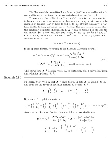
Example 3.8.1
Problem: Start with A and A −1 given below. Update A by adding 1 to a 21 ,
and then use the Sherman–Morrison formula to update A −1 :

12 −1 3 −2
A = and A = .
13 −1 1
Solution: The updated matrix is

12 12 00 12 0 T
B = = + = + (1 0) = A + e 2 e .
1
23 13 10 13 1
Applying the Sherman–Morrison formula yields the updated inverse
T
A −1 e 2 e A −1 −1 [A −1 ] ∗2 [A −1 ] 1∗
1
−1
−1
B = A − = A −
T
1+ e A −1 1+[A −1 ] 12
1 e 2

−2
(3 −2)
3 −2 1 −3 2
= − = .
−1 1 1 − 2 2 −1