Page 135 - Matrix Analysis & Applied Linear Algebra

3.8 Inverses of Sums and Sensitivity129

change (or error) in A. Therefore, we must consider A and the associated linear
system to be ill conditioned.
A Rule of Thumb. If Gaussian elimination with partial pivoting is used to
solve a well-scaled nonsingular system Ax = b using t -digit floating-point
arithmetic, then, assuming no other source of error exists, it can be argued that
p
when κ is of order 10 , the computed solution is expected to be accurate to
at least t − p significant digits, more or less. In other words, one expects to
lose roughly p significant figures. For example, if Gaussian elimination with 8-
digit arithmetic is used to solve the 2 × 2 system given above, then only about
t − p =8 − 6 = 2 significant figures of accuracy should be expected. This
doesn’t preclude the possibility of getting lucky and attaining a higher degree of
accuracy—it just says that you shouldn’t bet the farm on it.

The complete story of conditioning has not yet been told. As pointed out ear-
lier, it’s about three times more costly to compute A −1 than to solve Ax = b,
so it doesn’t make sense to compute A −1 just to estimate the condition of A.
Questions concerning condition estimation without explicitly computing an in-
verse still need to be addressed. Furthermore, liberties allowed by using the ≈
<
and ∼ symbols produce results that are intuitively correct but not rigorous.
Rigor will eventually be attained—see Example 5.12.1on p. 414.
Exercises for section 3.8

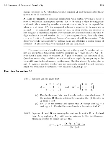
3.8.1. Suppose you are given that

   
20 −1 10 1
A =  −11 1  and A −1 =  01 −1  .
−10 1 10 2

(a) Use the Sherman–Morrison formula to determine the inverse of
the matrix B that is obtained by changing the (3, 2)-entry in
A from0to2.
(b) Let C be the matrix that agrees with A except that c 32 =2
and c 33 =2. Use the Sherman–Morrison formula to find C −1 .

3.8.2. Suppose A and B are nonsingular matrices in which B is obtained
from A by replacing A ∗j with another column b. Use the Sherman–
Morrison formula to derive the fact that
−1 −1
A b − e j [A ] j∗
B −1 = A −1 − .
[A −1 ] j∗ b