Page 137 - Matrix Analysis & Applied Linear Algebra

3.9 ElementaryMatrices and Equivalence 131
3.9 ELEMENTARY MATRICES AND EQUIVALENCE

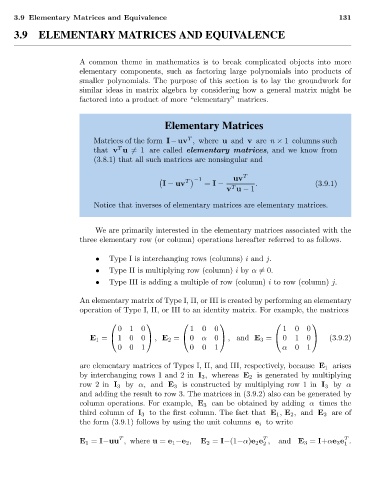
A common theme in mathematics is to break complicated objects into more
elementary components, such as factoring large polynomials into products of
smaller polynomials. The purpose of this section is to lay the groundwork for
similar ideas in matrix algebra by considering how a general matrix might be
factored into a product of more “elementary” matrices.

Elementary Matrices
T
Matrices of the form I−uv , where u and v are n × 1 columns such
T
that v u
= 1 are called elementary matrices, and we know from
(3.8.1) that all such matrices are nonsingular and

T −1 uv T
I − uv = I − . (3.9.1)
T
v u − 1
Notice that inverses of elementary matrices are elementary matrices.

We are primarily interested in the elementary matrices associated with the
three elementary row (or column) operations hereafter referred to as follows.

• Type I is interchanging rows (columns) i and j.
• Type II is multiplying row (column) i by α
=0.
• Type III is adding a multiple of row (column) i to row (column) j.

An elementary matrix of Type I, II, or III is created by performing an elementary
operation of Type I, II, or III to an identity matrix. For example, the matrices

     
010 1 0 0 1 0 0
E 1 =  100  , E 2 =  0 α 0  , and E 3 =  0 1 0  (3.9.2)
001 0 0 1 α 01

are elementary matrices of Types I, II, and III, respectively, because E 1 arises
by interchanging rows 1 and 2 in I 3 , whereas E 2 is generated by multiplying
row2in I 3 by α, and E 3 is constructed by multiplying row 1 in I 3 by α
and adding the result to row 3. The matrices in (3.9.2) also can be generated by
column operations. For example, E 3 can be obtained by adding α times the
third column of I 3 to the first column. The fact that E 1 , E 2 , and E 3 are of
the form (3.9.1) follows by using the unit columns e i to write

T
T
T
E 1 = I−uu , where u = e 1 −e 2 , E 2 = I−(1−α)e 2 e , and E 3 = I+αe 3 e .
2 1