Page 147 - Matrix Analysis & Applied Linear Algebra

3.10 The LU Factorization 141
3.10 THE LU FACTORIZATION

We have now come full circle, and we are back to where the text began—solving
a nonsingular system of linear equations using Gaussian elimination with back
substitution. This time, however, the goal is to describe and understand the
process in the context of matrices.
If Ax = b is a nonsingular system, then the object of Gaussian elimination
is to reduce A to an upper-triangular matrix using elementary row operations.
If no zero pivots are encountered, then row interchanges are not necessary, and
the reduction can be accomplished by using only elementary row operations of
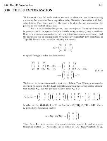
Type III. For example, consider reducing the matrix

 
2 2 2
A =  4 7 7 
61822

to upper-triangular form as shown below:

   
2 2 2 2 2 2
 4 7 7  R 2 − 2R 1 −→  0 3 3 
61822 R 3 − 3R 1 01216 R 3 − 4R 2
(3.10.1)
 
222
−→  033  = U.
004

We learned in the previous section that each of these Type III operations can be
executed by means of a left-hand multiplication with the corresponding elemen-
tary matrix G i , and the product of all of these G i ’s is

       
1 0 0 100 100 1 0 0
G 3 G 2 G 1 =  0 1 0   010   −210  =  −2 1 0  .
0 −41 −301 001 5 −41

−1 −1 −1
In other words, G 3 G 2 G 1 A = U, so that A = G 1 G 2 G 3 U = LU, where
L is the lower-triangular matrix
 
100
L = G −1 G −1 G −1 =  210  .
1 2 3
341
Thus A = LU is a product of a lower-triangular matrix L and an upper-
triangular matrix U. Naturally, this is called an LU factorization of A.