Page 151 - Matrix Analysis & Applied Linear Algebra

3.10 The LU Factorization 145
Example 3.10.1

Once L and U are known, there is usually no need to manipulate with A. This
together with the fact that the multipliers used in Gaussian elimination occur in
just the right places in L means that A can be successively overwritten with the
information in L and U as Gaussian elimination evolves. The rule is to store
the multiplier ' ij in the position it annihilates—namely, the (i, j)-position of
the array. For a 3 × 3 matrix, the result looks like this:
   
a 11 a 12 a 13 u 11 u 12 u 13
T ype III operations
  −−−−−−−−→   .
a 21 a 22 a 23 ' 21 u 22 u 23
a 31 a 32 a 33 ' 31 ' 32 u 33
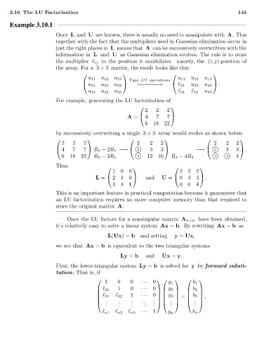
For example, generating the LU factorization of
 
2 2 2
A =  4 7 7 
61822
by successively overwriting a single 3 × 3 array would evolve as shown below:
     
2 2 2 2 2 2 2 2 2

 4 7 7  R 2 − 2R 1 −→  2 3 3  −→  2 3 3  .
61822 R 3 − 3R 1 12 16 R 3 − 4R 2 4
3
3
4
Thus
   
100 222
L =  210  and U =  033  .
341 004
This is an important feature in practical computation because it guarantees that
an LU factorization requires no more computer memory than that required to
store the original matrix A.
Once the LU factors for a nonsingular matrix A n×n have been obtained,
it’s relatively easy to solve a linear system Ax = b. By rewriting Ax = b as
L(Ux)= b and setting y = Ux,
we see that Ax = b is equivalent to the two triangular systems

Ly = b and Ux = y.
First, the lower-triangular system Ly = b is solved for y by forward substi-
tution. That is, if
1 0 0 ··· 0 y 1 b 1
     
1 0
 ' 21 ··· 0   y 2   b 2 
     
 ' 31 ' 32 1 ··· 0   y 3  =  b 3  ,
 . . . . .   .   . 
 . . . .  . 
. . . . . .   .  .
.
' n1 ' n2 ' n3 ··· 1 y n b n