Page 148 - Matrix Analysis & Applied Linear Algebra

142 Chapter 3 Matrix Algebra

Observe that U is the end product of Gaussian elimination and has the
pivots on its diagonal, while L has 1’s on its diagonal. Moreover, L has the
remarkable property that below its diagonal, each entry ' ij is precisely the
multiplier used in the elimination (3.10.1) to annihilate the (i, j)-position.
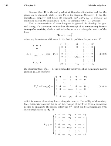
This is characteristic of what happens in general. To develop the gen-
eral theory, it’s convenient to introduce the concept of an elementary lower-
triangular matrix, which is defined to be an n × n triangular matrix of the
form
T
T k = I − c k e ,
k
where c k is a column with zeros in the first k positions. In particular, if
 
10 0 0 ··· 0
0
  ···
 01 ··· 0 0 ··· 0 
 0   . . . . . . 
 .
 .   . . . . . . . . . . 
.
 .  . 
 , then T k =  00 ··· 1 0 ··· 0  . (3.10.2)
   
c k = 

 µ k+1   00 ··· −µ k+1 1 
 .  ··· 0 
.  . . . . .
 .   . . . . . . 
. . . . . . . 
µ n
00 ··· −µ n 0 ··· 1
T
By observing that e c k =0, the formula for the inverse of an elementary matrix
k
given in (3.9.1) produces
 
10 ··· 0 0 ··· 0
 01 ··· 0 0 ··· 0 
 . . . . . . . . . . . 

 . . . . . . 
. 
−1 T  
T = I + c k e =  00 ··· 1 0 ··· 0  , (3.10.3)
k k
 00 ··· µ k+1 1 ··· 0 


 . . . . . . 
 . . . . . . 
. . . . . .
00 ··· µ n 0 ··· 1
which is also an elementary lower-triangular matrix. The utility of elementary
lower-triangular matrices lies in the fact that all of the Type III row operations
needed to annihilate the entries below the k th pivot can be accomplished with
one multiplication by T k . If
 
∗∗· · · α 1 ∗· · · ∗
 0 ∗· · · α 2 ∗· · · ∗ 
 . . . . .
 . . . . . . 
 . . . . . . 
. 
A k−1 =  00 ··· α k ∗· · · ∗ 


 00 ··· α k+1 ∗· · · ∗ 


 . . . . . 
 . . . . . .
. . . . . . . 
00 ··· α n ∗· · · ∗