Page 319 - Matrix Analysis & Applied Linear Algebra

5.5 Gram–Schmidt Procedure 315

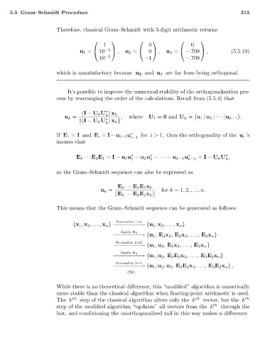
Therefore, classical Gram–Schmidt with 3-digit arithmetic returns

     
1 0 0
u 1 =  10 −3  , u 2 =  0  , u 3 =  −.709  , (5.5.10)
10 −3 −1 −.709

which is unsatisfactory because u 2 and u 3 are far from being orthogonal.

It’s possible to improve the numerical stability of the orthogonalization pro-
cess by rearranging the order of the calculations. Recall from (5.5.4) that

∗
(I − U k U ) x k
k
u k = , where U 1 = 0 and U k = u 1 | u 2 |···| u k−1 .
∗
(I − U k U ) x k
k
If E 1 = I and E i = I − u i−1 u ∗ i−1 for i> 1, then the orthogonality of the u i ’s
insures that
∗
E k ··· E 2 E 1 = I − u 1 u − u 2 u −· · · − u k−1 u ∗ k−1 = I − U k U ,
∗
∗
2
1
k
so the Gram–Schmidt sequence can also be expressed as
E k ··· E 2 E 1 x k
u k = for k =1, 2,...,n.
E k ··· E 2 E 1 x k
This means that the Gram–Schmidt sequence can be generated as follows:

Normalize 1-st
{x 1 , x 2 ,..., x n } −−−−−−−−−→{u 1 , x 2 ,..., x n }
Apply E 2
−−−−−−−−−→{u 1 , E 2 x 2 , E 2 x 3 ,. . . , E 2 x n }
Normalize 2-nd
−−−−−−−−−→{u 1 , u 2 , E 2 x 3 ,. . . , E 2 x n }
Apply E 3
−−−−−−−−−→{u 1 , u 2 , E 3 E 2 x 3 , ..., E 3 E 2 x n }
Normalize 3-rd
−−−−−−−−−→{u 1 , u 2 , u 3 , E 3 E 2 x 4 ,..., E 3 E 2 x n } ,
etc.

While there is no theoretical difference, this “modified” algorithm is numerically
more stable than the classical algorithm when floating-point arithmetic is used.
The k th step of the classical algorithm alters only the k th vector, but the k th
step of the modified algorithm “updates” all vectors from the k th through the
last, and conditioning the unorthogonalized tail in this way makes a difference.