Page 318 - Matrix Analysis & Applied Linear Algebra

314 Chapter 5 Norms, Inner Products, and Orthogonality

Linear Systems and the QR Factorization
If rank (A m×n )= n, and if A = QR is the QR factorization, then the
solution of the nonsingular triangular system
T
Rx = Q b (5.5.9)

is either the solution or the least squares solution of Ax = b depending
on whether or not Ax = b is consistent.

It’s worthwhile to reemphasize that the QR approach to the least squares prob-
T
T
lem obviates the need to explicitly compute the product A A. But if A A is
T
T
ever needed, it is retrievable from the factorization A A = R R. In fact, this
T
is the Cholesky factorization of A A as discussed in Example 3.10.7, p. 154.
The Gram–Schmidt procedure is a powerful theoretical tool, but it’s not a
good numerical algorithm when implemented in the straightforward or “classi-
cal” sense. When floating-point arithmetic is used, the classical Gram–Schmidt
algorithm applied to a set of vectors that is not already close to being an orthog-
onal set can produce a set of vectors that is far from being an orthogonal set. To
see this, consider the following example.
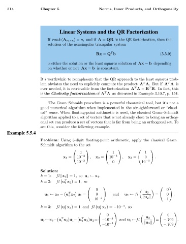
Example 5.5.4

Problem: Using 3-digit floating-point arithmetic, apply the classical Gram–
Schmidt algorithm to the set
     
1 1 1
x 1 =  10 −3  , x 2 =  10 −3  , x 3 =  0  .
10 −3 0 10 −3
Solution:
k =1: fl x 1 =1, so u 1 ← x 1 .

T
k =2: fl u x 2 =1, so
1
   
0 0
T u 2
u 2 ← x 2 − u x 2 u 1 =  0  and u 2 ← fl =  0  .
1
−10 −3 u 2 −1
T T −3
k =3: fl u x 3 =1 and fl u x 3 = −10 , so
1
2
   
0 0
T T u 3
u 3 ←x 3 − u x 3 u 1 − u x 3 u 2 =  −10 −3  and u 3 ←fl =  −.709  .
2
1
−10 −3 u 3 −.709