Page 316 - Matrix Analysis & Applied Linear Algebra

312 Chapter 5 Norms, Inner Products, and Orthogonality
 
0
a 1
k =1: r 11 ← a 1 =5 and q 1 ← =  3/5 
r 11
4/5
T
k =2: r 12 ← q a 2 =25
1  
−20
q 2 ← a 2 − r 12 q 1 =  12 
−9
 
−20
1
q 2
r 22 ← q 2 =25 and q 2 ← =  12 
r 22 25
−9
T
T
k =3: r 13 ← q a 3 = −4 and r 23 ← q a 3 =10
1 2
 
−15
2
q 3 ← a 3 − r 13 q 1 − r 23 q 2 =  −16 
5
12
 
−15
1
q 3
r 33 ← q 3 =10 and q 3 ← =  −16 
r 33 25
12
Therefore,
   
0 −20 −15 525 −4
1
Q =  15 12 −16  and R =  025 10  .
25
20 −9 12 0 0 10
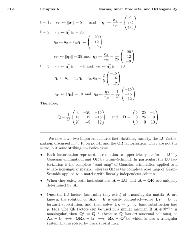
We now have two important matrix factorizations, namely, the LU factor-
ization, discussed in §3.10 on p. 141 and the QR factorization. They are not the
same, but some striking analogies exist.
• Each factorization represents a reduction to upper-triangular form—LU by
Gaussian elimination, and QR by Gram–Schmidt. In particular, the LU fac-
torization is the complete “road map” of Gaussian elimination applied to a
square nonsingular matrix, whereas QR is the complete road map of Gram–
Schmidt applied to a matrix with linearly independent columns.
• When they exist, both factorizations A = LU and A = QR are uniquely
determined by A.

• Once the LU factors (assuming they exist) of a nonsingular matrix A are
known, the solution of Ax = b is easily computed—solve Ly = b by
forward substitution, and then solve Ux = y by back substitution (see
n×n
p. 146). The QR factors can be used in a similar manner. If A ∈ is
nonsingular, then Q T = Q −1 (because Q has orthonormal columns), so
T
Ax = b ⇐⇒ QRx = b ⇐⇒ Rx = Q b, which is also a triangular
system that is solved by back substitution.