Page 320 - Matrix Analysis & Applied Linear Algebra

316 Chapter 5 Norms, Inner Products, and Orthogonality

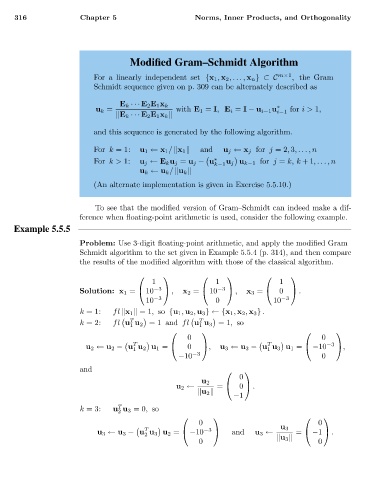
Modified Gram–Schmidt Algorithm

m×1
Fora linearly independent set {x 1 , x 2 ,..., x n }⊂C , the Gram–
Schmidt sequence given on p. 309 can be alternately described as

E k ··· E 2 E 1 x k
u k = with E 1 = I, E i = I − u i−1 u ∗ i−1 for i> 1,
E k ··· E 2 E 1 x k
and this sequence is generated by the following algorithm.

For k =1: u 1 ← x 1 / x 1 and u j ← x j for j =2, 3,...,n

For k> 1: u j ← E k u j = u j − u ∗ k−1 u j u k−1 for j = k, k +1,...,n
u k ← u k / u k
(An alternate implementation is given in Exercise 5.5.10.)

To see that the modified version of Gram–Schmidt can indeed make a dif-
ference when floating-point arithmetic is used, consider the following example.
Example 5.5.5

Problem: Use 3-digit floating-point arithmetic, and apply the modified Gram–
Schmidt algorithm to the set given in Example 5.5.4 (p. 314), and then compare
the results of the modified algorithm with those of the classical algorithm.

     
1 1 1
Solution: x 1 =  10 −3  , x 2 =  10 −3  , x 3 =  0  .
10 −3 0 10 −3
k =1: fl x 1 =1, so {u 1 , u 2 , u 3 }←{x 1 , x 2 , x 3 } .

T
T
k =2: fl u u 2 =1 and fl u u 3 =1, so
1 1
   
0 0
T T
u 2 ← u 2 − u u 2 u 1 =  0  , u 3 ← u 3 − u u 3 u 1 =  −10 −3  ,
1
1
−10 −3 0
and  
0
u 2
u 2 ← =  0  .
u 2
−1
T
k =3: u u 3 =0, so
2
   
0 0
T u 3
u 3 ← u 3 − u u 3 u 2 =  −10 −3  and u 3 ← =  −1  .
2
0 u 3 0