Page 378 - Matrix Analysis & Applied Linear Algebra

374 Chapter 5 Norms, Inner Products, and Orthogonality

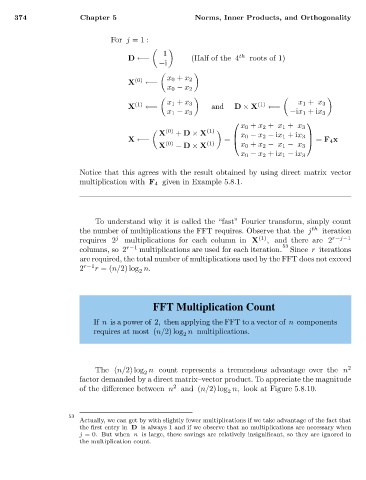
For j =1:

1 th
D ←− (Half of the 4 roots of 1)
−i

X (0) ←− x 0 + x 2
x 0 − x 2

X (1) ←− x 1 + x 3 and D × X (1) ←− x 1 + x 3
x 1 − x 3 −ix 1 +ix 3
 
x 0 + x 2 + x 1 + x 3
(0) (1)
X + D × X
 x 0 − x 2 − ix 1 +ix 3 
X ←− (0) (1) =   = F 4 x
X − D × X x 0 + x 2 − x 1 − x 3
x 0 − x 2 +ix 1 − ix 3
Notice that this agrees with the result obtained by using direct matrix–vector
multiplication with F 4 given in Example 5.8.1.

To understand why it is called the “fast” Fourier transform, simply count
the number of multiplications the FFT requires. Observe that the j th iteration
requires 2 j multiplications for each column in X (1) , and there are 2 r−j−1
columns, so 2 r−1 multiplications are used for each iteration. 53 Since r iterations
are required, the total number of multiplications used by the FFT does not exceed
2 r−1 r =(n/2) log n.
2

FFT Multiplication Count
If n is a power of 2, then applying the FFT to a vector of n components
requires at most (n/2) log n multiplications.
2

The (n/2) log n count represents a tremendous advantage over the n 2
2
factor demanded by a direct matrix–vector product. To appreciate the magnitude
2
of the difference between n and (n/2) log n, look at Figure 5.8.10.
2
53
Actually, we can get by with slightly fewer multiplications if we take advantage of the fact that
the first entry in D is always 1 and if we observe that no multiplications are necessary when
j =0. But when n is large, these savings are relatively insignificant, so they are ignored in
the multiplication count.