Page 376 - Matrix Analysis & Applied Linear Algebra

372 Chapter 5 Norms, Inner Products, and Orthogonality

positions. Then each group was broken into two more groups by again separating
the entries in the even positions from those in the odd positions.

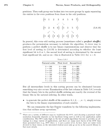
0 1 2 3 4 5 6 7

0 2 4 6 1 3 5 7 (5.8.19)

04 26 15 37

In general, this even–odd sorting process (sometimes called a perfect shuffle)
produces the permutation necessary to initiate the algorithm. A clever way to
perform a perfect shuffle is to use binary representations and observe that the
first level of sorting in (5.8.19) is determined according to whether the least
significant bit is 0 or 1, the second level of sorting is determined by the second
least significant bit, and so on—this is illustrated in Table 5.8.1 for n =8.

Table 5.8.1
Natural order First level Second level
0 ↔ 000 0 ↔ 000 0 ↔ 000
1 ↔ 001 2 ↔ 010 4 ↔ 100
2 ↔ 010 4 ↔ 100 2 ↔ 010
3 ↔ 011 6 ↔ 110 6 ↔ 110
4 ↔ 100 1 ↔ 001 1 ↔ 001
5 ↔ 101 3 ↔ 011 5 ↔ 101
6 ↔ 110 5 ↔ 101 3 ↔ 011
7 ↔ 111 7 ↔ 111 7 ↔ 111

But all intermediate levels in this sorting process can be eliminated because
something very nice occurs. Examination of the last column in Table 5.8.1 reveals
that the binary bits in the perfect shuffle ordering are exactly the reversal of the
binary bits in the natural ordering. In other words,

• to generate the perfect shuffle of the numbers 0, 1, 2,...,n−1, simply reverse
the bits in the binary representation of each number.
We can summarize the fast Fourier transform by the following implementa-
52
tion that utilizes array operations.
52
There are a variety of different ways to implement the FFT, and choosing a practical imple-
mentation frequently depends on the hardware being used as well as the application under
consideration. The FFT ranks high on the list of useful algorithms because it provides an ad-
vantage in a large variety of applications, and there are many more facets of the FFT than
those presented here (e.g., FFT when n is not a power of 2). In fact, there are entire texts
devoted to these issues, so the interested student need only go as far as the nearest library to
find more details.