
Page 379 - Matrix Analysis & Applied Linear Algebra
P. 379
5.8 Discrete Fourier Transform 375
300000
200000 f(n) = n 2
100000
f(n) = (n/2) log n
2
0
0 128 256 512
n
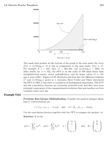
Figure 5.8.10
The small dark portion at the bottom of the graph is the area under the curve
2
f(n)=(n/2) log n—it is tiny in comparison to the area under f(n)= n .
2
2
For example, if n = 512, then n = 262, 144, but (n/2) log n = 2304. In
2
other words, for n = 512, the FFT is on the order of 100 times faster than
straightforward matrix–vector multiplication, and for larger values of n, the
gap is even wider—Figure 5.8.10 illustrates just how fast the difference between
2
n and (n/2) log n grows as n increases. Since Cooley and Tukey introduced
2
the FFT in 1965, it has risen to a position of fundamental importance. The FFT
and the convolution theorem are extremely powerful tools, and they have been
principal components of the computational revolution that now touches our lives
countless times each day.
Example 5.8.6
Problem: Fast Integer Multiplication. Consider two positive integers whose
base-b representations are
and d =(δ n−1 δ n−2 ··· δ 1 δ 0 ) b .
c =(γ n−1 γ n−2 ··· γ 1 γ 0 ) b
Use the convolution theorem together with the FFT to compute the product cd.
Solution: If we let
γ 0 δ 0
n−1 n−1
γ 1 δ 1
k
k
p(x)= γ k x , q(x)= δ k x , c = . , and d = . ,
. . .
k=0 k=0 .
γ n−1 δ n−1