Page 375 - Matrix Analysis & Applied Linear Algebra

5.8 Discrete Fourier Transform 371

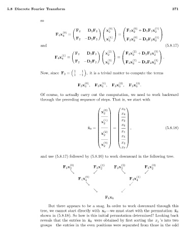
so

   
(0) (0) (1)
F 2 D 2 F 2 x 2 F 2 x 2 + D 2 F 2 x 2
(0)
F 4 x 4 =   =  
F 2 −D 2 F 2 x (1) F 2 x (0) − D 2 F 2 x (1)
2
2
2
and (5.8.17)
   
(2) (2) (3)
F 2 D 2 F 2 x 2 F 2 x 2 + D 2 F 2 x 2
(1)
F 4 x =   =   .
4 (3) (2) (3)
F 2 −D 2 F 2 x F 2 x − D 2 F 2 x
2 2 2

1 1
Now, since F 2 = , it is a trivial matter to compute the terms
1 −1
(0) (1) (2) (3)
F 2 x , F 2 x , F 2 x , F 2 x .
2 2 2 2
Of course, to actually carry out the computation, we need to work backward
through the preceding sequence of steps. That is, we start with
   
x 0
(0)
x
 2   x 4 
   
 (1)   
 x   x 2 
 2   
   x 6 
˜ x 8 =   =   , (5.8.18)
 (2)   x 1 
 x   
 2   x 5 
   
   
(3) x 3
x
2
x 7
and use (5.8.17) followed by (5.8.16) to work downward in the following tree.
(0) (1) (2) (3)
F 2 x F 2 x F 2 x F 2 x
2 2 2 2

(0) (1)
F 4 x F 4 x
4 4

F 8 x 8
But there appears to be a snag. In order to work downward through this
tree, we cannot start directly with x 8 —we must start with the permutation ˜ x 8
shown in (5.8.18). So how is this initial permutation determined? Looking back
reveals that the entries in ˜ x 8 were obtained by first sorting the x j ’s into two
groups—the entries in the even positions were separated from those in the odd