Page 370 - Matrix Analysis & Applied Linear Algebra

366 Chapter 5 Norms, Inner Products, and Orthogonality

If
   
α 0 β 0
 α 1   β 1 
a =  .  and b =  .  ,
 . .   . . 
α n−1 n×1 β n−1 n×1

then the vector
 
α 0 β 0
 
α 0 β 1 + α 1 β 0
 
 
 
 α 0 β 2 + α 1 β 1 + α 2 β 0 
.
 
a b= . .  (5.8.10)
 
 
 α n−2 β n−1 + α n−1 β n−2 
 
 α n−1 β n−1 
0
2n×1
is called the convolution of a and b. The 0 in the last position is for con-
venience only—it makes the size of the convolution twice the size of the origi-
nal vectors, and this provides a balance in some of the formulas involving con-
volution. Furthermore, it is sometimes convenient to pad a and b with n
additional zeros to consider them to be vectors with 2n components. Setting
α n = ··· = α 2n−1 = β n = ··· = β 2n−1 =0 allows us to write the k th entry in
a b as
k

[a b] k = α j β k−j for k =0, 1, 2,..., 2n − 1.
j=0
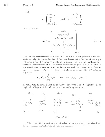
A visual way to form a b is to “slide” the reversal of b “against” a as
depicted in Figure 5.8.9, and then sum the resulting products.

β n−1 β n−1 α 0
. β n−1 . α 0 .
. . . . .
. . . . .
. .
β 1 α 0 ×β 2 α n−2
α 0 ×β 1 α n−2 ×β n−1
α 0 ×β 0 α 1 ×β 1 ··· α n−1 ×β n−1
α 1 ×β 0 α n−1 ×β n−2
α 1 . α 2 ×β 0 . β n−2
. . . . . .
. . . .
. . .
α n−1 β 0
α n−1 α n−1 β 0
Figure 5.8.9
The convolution operation is a natural occurrence in a variety of situations,
and polynomial multiplication is one such example.