Page 369 - Matrix Analysis & Applied Linear Algebra

5.8 Discrete Fourier Transform 365

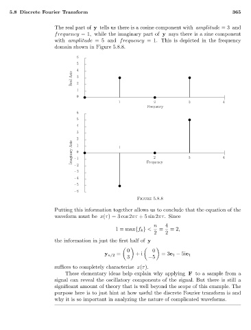
The real part of y tells us there is a cosine component with amplitude =3 and
frequency =1, while the imaginary part of y says there is a sine component
with amplitude =5 and frequency =1. This is depicted in the frequency
domain shown in Figure 5.8.8.
6
5
4
Real Axis 3 2

1
0
1 2 3 4
Frequency
6
5
4
3
2 1
Imaginary Axis -1 0 1 2 3 4

-2 Frequency
-3
-4
-5
-6
Figure 5.8.8
Putting this information together allows us to conclude that the equation of the
waveform must be x(τ)=3 cos 2πτ +5 sin 2πτ. Since
n 4
1= max{f k } < = =2,
2 2
the information in just the first half of y

0 0
y n/2 = +i =3e 1 − 5ie 1
3 −5
suffices to completely characterize x(τ).
These elementary ideas help explain why applying F to a sample from a
signal can reveal the oscillatory components of the signal. But there is still a
significant amount of theory that is well beyond the scope of this example. The
purpose here is to just hint at how useful the discrete Fourier transform is and
why it is so important in analyzing the nature of complicated waveforms.