Page 364 - Matrix Analysis & Applied Linear Algebra

360 Chapter 5 Norms, Inner Products, and Orthogonality

It seems reasonable to expect that the signal should have oscillatory components
together with some random noise contamination. That is, we expect the signal
to have the form

y(τ)= α k cos 2πf k τ + β k sin 2πf k τ + Noise.
k
But due to the noise contamination, the oscillatory nature of the signal is only
barely apparent—the characteristic “chop-a chop-a chop-a” is not completely
clear. To reveal the oscillatory components, the magic of the Fourier transform
is employed. Let x be the vector obtained by sampling the signal at n equally
spaced points between time τ =0 and τ =1 ( n = 512 in our case), and let

y =(2/n)F n x = a +ib, where a =(2/n)Re (F n x) and b =(2/n)Im (F n x) .

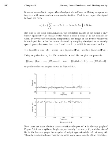
Using only the first n/2= 256 entries in a and ib, we plot the points in

{(0,a 0 ), (1,a 1 ),. . . , (255,a 255 )} and {(0, ib 0 ), (1, ib 1 ),. . . , (255, ib 255 )}
to produce the two graphs shown in Figure 5.8.4.

1.5
1
Real Axis 0.5

0

-0.5
0 50 100 150 200 250 300
Frequency
0.5
0
Imaginary Axis -0.5

-1
-1.5
-2
0 50 100 150 200 250 300
Frequency
Figure 5.8.4
Now there are some obvious characteristics—the plot of a in the top graph of
Figure 5.8.4 has a spike of height approximately 1 at entry 80, and the plot of
ib in the bottom graph has a spike of height approximately −2at entry 50.
These two spikes indicate that the signal is made up primarily of two oscillatory