Page 361 - Matrix Analysis & Applied Linear Algebra

5.8 Discrete Fourier Transform 357

Furthermore, the fact that

k
k
ξ k 1+ ξ + ξ 2k + ··· + ξ (n−2)k + ξ (n−1)k = ξ + ξ 2k + ··· + ξ (n−1)k +1
k 2k (n−1)k k
implies 1+ ξ + ξ + ··· + ξ 1 − ξ = 0 and, consequently,
k
k
1+ ξ + ξ 2k + ··· + ξ (n−1)k = 0 whenever ξ =1. (5.8.2)

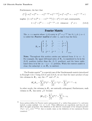
Fourier Matrix
The n × n matrix whose (j, k)-entry is ξ jk = ω −jk for 0 ≤ j, k ≤ n−1
is called the Fourier matrix of order n, and it has the form

11 1 ··· 1
 
 1 ξ ξ 2 ··· ξ n−1 

F n =  1 ξ 2 ξ 4 ··· ξ n−2  .


 . . . . . . . . . . 
. . . . . 
1 ξ n−1 ξ n−2 ··· ξ
n×n
Note. Throughout this section entries are indexed from 0 to n − 1.
For example, the upper left-hand entry of F n is considered to be in the
(0, 0)position (rather than the (1, 1)position), and the lower right-
hand entry is in the (n − 1,n − 1)position. When the context makes it
clear, the subscript n on F n is omitted.

50
The Fourier matrix is a special case of the Vandermonde matrix introduced
in Example 4.3.4. Using (5.8.1)and (5.8.2), we see that the inner product of any
th
two columns in F n , say, the r th and s ,is
n−1 n−1 n−1
−jr js j(s−r)
jr js
∗
F F ∗s = ξ ξ = ξ ξ = ξ =0.
∗r
j=0 j=0 j=0
In other words, the columns in F n are mutually orthogonal. Furthermore, each
√
column in F n has norm n because
n−1 n−1
2 jk 2
F ∗k = |ξ | = 1= n,
2
j=0 j=0
50
Some authors define the Fourier matrix using powers of ω rather than powers of ξ, and some
√
include a scalar multiple 1/n or 1/ n. These differences are superficial, and they do not
affect the basic properties. Our definition is the discrete counterpart of the integral operator

∞
F(f)= x(t)e −i2πft dt that is usually taken as the definition of the continuous Fourier
−∞
transform.