Page 371 - Matrix Analysis & Applied Linear Algebra

5.8 Discrete Fourier Transform 367
Example 5.8.4
n−1 k n−1 k
Polynomial Multiplication. For p(x)= α k x ,q(x)= β k x , let
k=0 k=0
T T
a =( α 0 α 1 ··· α n−1 ) and b =( β 0 β 1 ··· β n−1 ) . The product
2
p(x)q(x)= γ 0 + γ 1 x + γ 2 x + ··· + γ 2n−2 x 2n−2 is a polynomial of degree 2n − 2
in which γ k is simply the k th component of the convolution a b because
 
2n−2 k 2n−2
k k
p(x)q(x)=  α j β k−j x = [a b] k x . (5.8.11)

k=0 j=0 k=0
In other words, polynomial multiplication and convolution are equivalent opera-
tions, so if we can devise an efficient way to perform a convolution, then we can
efficiently multiply two polynomials, and conversely.
There are two facets involved in efficiently performing a convolution. The
first is the realization that the discrete Fourier transform has the ability to
convert a convolution into an ordinary product, and vice versa. The second is
the realization that it’s possible to devise a fast algorithm to compute a discrete
Fourier transform. These two facets are developed below.

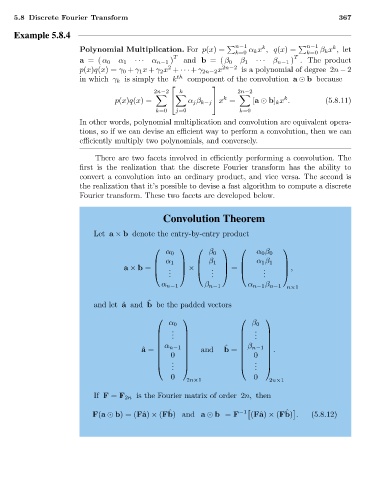
Convolution Theorem
Let a × b denote the entry-by-entry product

     
α 0 β 0 α 0 β 0
α 1 β 1
 α 1   β 1   
a × b =  .  ×  .  =  .  ,
. . .
 .   .   . 
α n−1 β n−1 α n−1 β n−1
n×1
ˆ
and let ˆ a and b be the padded vectors
   
α 0 β 0
. .
 .   . 
 .   . 
   
 α n−1  ˆ  β n−1 
ˆ a =   and b =  .
0
   0 
. .
   
. .
 .   . 
0 0
2n×1 2n×1
If F = F 2n is the Fourier matrix of order 2n, then

ˆ
ˆ
F(a b)=(Fˆ a) × (Fb) and a b = F −1 (Fˆ a) × (Fb) . (5.8.12)