Page 74 - Matrix Analysis & Applied Linear Algebra

2.5 Nonhomogeneous Systems 67

That is, the two solutions differ only in the fact that the latter contains the
constant ξ i . Consider organizing the expressions (2.5.5) and (2.5.6) so as to
construct the respective general solutions. If the general solution of the homoge-
neous system has the form

h n−r ,
x = x f 1 h 1 + x f 2 h 2 + ··· + x f n−r
then it is apparent that the general solution of the nonhomogeneous system must
have a similar form

h n−r (2.5.7)
x = p + x f 1 h 1 + x f 2 h 2 + ··· + x f n−r
in which the column p contains the constants ξ i along with some 0’s—the ξ i ’s
occupy positions in p that correspond to the positions of the basic columns, and
0’s occupy all other positions. The column p represents one particular solution
to the nonhomogeneous system because it is the solution produced when the free
=0.
variables assume the values x f 1 = x f 2 = ··· = x f n−r
Example 2.5.1

Problem: Determine the general solution of the following nonhomogeneous sys-
tem and compare it with the general solution of the associated homogeneous
system:
x 1 + x 2 +2x 3 +2x 4 + x 5 =1,
2x 1 +2x 2 +4x 3 +4x 4 +3x 5 =1,
2x 1 +2x 2 +4x 3 +4x 4 +2x 5 =2,
3x 1 +5x 2 +8x 3 +6x 4 +5x 5 =3.

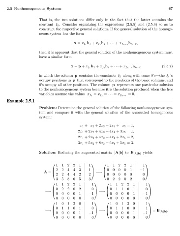
Solution: Reducing the augmented matrix [A|b]to E [A|b] yields

11221 1 11221 1
   
 22443 1   00001 −1 
22442 2  −→  00000 0 
A = 
35865 3 02202 0
11221 1 11221 1
   
 02202 0   01101 0 
00001 −1  −→  00001 −1 
−→ 
00000 0 00000 0
10120 1 10120 1
   
 01101 0   01100 1 
00001 −1 00001 −1
−→   −→   = E [A|b] .
00000 0 00000 0