Page 82 - Matrix Analysis & Applied Linear Algebra

2.6 Electrical Circuits 75

There are 4 additional loops that also produce loop equations thereby mak-
ing a total of 11 equations (4 nodal equations and 7 loop equations) in 6 un-
knowns. Although this appears to be a rather general 11 × 6 system of equations,
it really is not. If the circuit is in a state of equilibrium, then the physics of the
situation dictates that for each set of EMFs E k , the corresponding currents
I k must be uniquely determined. In other words, physics guarantees that the
11 × 6 system produced by applying the two Kirchhoff rules must be consistent
and possess a unique solution.
Suppose that [A|b] represents the augmented matrix for the 11 × 6 system
generated by Kirchhoff’s rules. From the results in §2.5, we know that the system
has a unique solution if and only if
rank (A) = number of unknowns = 6.

Furthermore, it was demonstrated in §2.3 that the system is consistent if and
only if
rank[A|b]= rank (A).
Combining these two facts allows us to conclude that
rank[A|b]=6
so that when [A|b] is reduced to E [A|b] , there will be exactly 6 nonzero rows
and 5 zero rows. Therefore, 5 of the original 11 equations are redundant in the
sense that they can be “zeroed out” by forming combinations of some particular
set of 6 “independent” equations. It is desirable to know beforehand which of
the 11 equations will be redundant and which can act as the “independent” set.
Notice that in using the node rule, the equation corresponding to node 4
is simply the negative sum of the equations for nodes 1, 2, and 3, and that the
first three equations are independent in the sense that no one of the three can
be written as a combination of any other two. This situation is typical. For a
general circuit with n nodes, it can be demonstrated that the equations for
the first n − 1 nodes are independent, and the equation for the last node is
redundant.
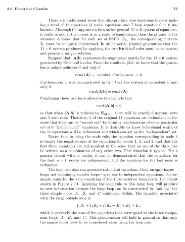
The loop rule also can generate redundant equations. Only simple loops—
loops not containing smaller loops—give rise to independent equations. For ex-
ample, consider the loop consisting of the three exterior branches in the circuit
shown in Figure 2.6.1. Applying the loop rule to this large loop will produce
no new information because the large loop can be constructed by “adding” the
three simple loops A, B, and C contained within. The equation associated
with the large outside loop is

I 1 R 1 + I 2 R 2 + I 4 R 4 = E 1 + E 2 + E 4 ,
which is precisely the sum of the equations that correspond to the three compo-
nent loops A, B, and C. This phenomenon will hold in general so that only
the simple loops need to be considered when using the loop rule.