Page 79 - Mechanical design of microresonators _ modeling and applications

0-07-145538-8_CH02_78_08/30/05

Basic Members: Lumped- and Distributed-Parameter Modeling and Design

78 Chapter Two

1.06
rm a 1.25
1.02
0.00001
α

t [m] 1.05
1
0.00005
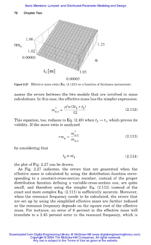
Figure 2.27 Effective mass ratio [Eq. (2.113)] as a function of thickness parameters.

assess the errors between the two models that are involved in mass
calculations. In this case, the effective mass has the simpler expression:
ȡlw(3t + t )
2
1
*
m a,e = 12 (2.112)
This equation, too, reduces to Eq. (2.49) when t ĺ t , which proves its
1
2
validity. If the mass ratio is analyzed
*
m a,e
rm = (2.113)
a
m
a,e
by considering that
t = Įt (2.114)
2 1
the plot of Fig. 2.27 can be drawn.
As Fig. 2.27 indicates, the errors that are generated when the
effective mass is calculated by using the distribution function corre-
sponding to a constant-cross-section member, instead of the proper
distribution function defining a variable-cross-section one, are quite
small; and therefore using the simpler Eq. (2.112) instead of the
exact and more complex Eq. (2.111) is sufficiently accurate. Moreover,
when the resonant frequency needs to be calculated, the errors that
are set up by using the simplified effective mass are further reduced
as the resonant frequency depends on the square root of the effective
mass. For instance, an error of 6 percent in the effective mass will
translate to a 2.45 percent error in the resonant frequency, which is

Downloaded from Digital Engineering Library @ McGraw-Hill (www.digitalengineeringlibrary.com)
Copyright © 2004 The McGraw-Hill Companies. All rights reserved.
Any use is subject to the Terms of Use as given at the website.