Page 362 - Mechanical Engineers' Handbook (Volume 2)

7 Simulation 353

7.2 Digital Simulation
Digital continuous-system simulation involves the approximate solution of a state-variable
model over successive time steps. Consider the general state-variable equation

˙ x(t) ƒ[x(t), u(t)]
to be simulated over the time interval t t t . The solution to this problem is based on
K
0
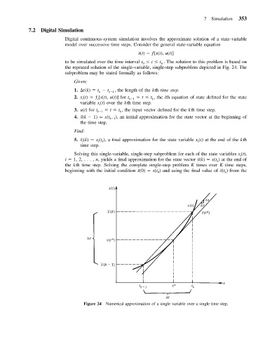
the repeated solution of the single-variable, single-step subproblem depicted in Fig. 24. The
subproblem may be stated formally as follows:
Given:
1. t(k) t t k 1 , the length of the kth time step.
k
2. x (t) ƒ [x(t), u(t)] for t k 1 t t , the ith equation of state defined for the state
i
i
k
variable x (t) over the kth time step.
i
3. u(t) for t k 1 t t , the input vector defined for the kth time step.
k
4. x(k 1) x(t k 1 ), an initial approximation for the state vector at the beginning of
˜
the time step.
Find:
˜
5. x (k) x (t ), a final approximation for the state variable x (t) at the end of the kth
k
i
i
i
time step.
Solving this single-variable, single-step subproblem for each of the state variables x (t),
i
i 1, 2,..., n, yields a final approximation for the state vector x˜(k) x(t ) at the end of
k
the kth time step. Solving the complete single-step problem K times over K time steps,
˜
beginning with the initial condition x(0) x(t ) and using the final value of x˜(t ) from the
k
0

Figure 24 Numerical approximation of a single variable over a single time step.