Page 364 - Mechanical Engineers' Handbook (Volume 2)

7 Simulation 355

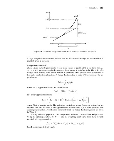
Figure 25 Geometric interpretation of the Euler method for numerical integration.

a large computational overhead and can lead to inaccuracies through the accumulation of
roundoff error at each step.
Runge–Kutta Methods
Runge–Kutta methods precompute two or more values of ƒ [x(t), u(t)] in the time step t k 1
i
˜
t t and use some weighted average of these values to calculate ƒ (k). The order of a
k
i
Runge–Kutta method refers to the number of derivative terms (or derivative calls) used in
the scalar single-step calculation. A Runge–Kutta routine of order N therefore uses the ap-
proximation
ƒ (k) w ƒ(k)
N
˜
i
j 1 j ij
where the N approximations to the derivative are
ƒ(k) ƒ[˜x(k 1), u(t k 1 )]
i1
i
(the Euler approximation) and
ƒ ƒ
˜ x(k 1) t t
j 1
j 1
b
jt il
ij
i
t 1 Ib ƒ, ut
k 1 t 1 jl
where I is the identity matrix. The weighting coefficients w and b are not unique, but are
jl
j
selected such that the error in the approximation is zero when x (t) is some specified Nth-
i
degree polynomial in t. Coefficients commonly used for Runge–Kutta integration are given
in Table 9.
Among the most popular of the Runge–Kutta methods is fourth-order Runge–Kutta.
Using the defining equations for N 4 and the weighting coefficients from Table 9 yields
the derivative approximation
˜
ƒ (k) ⁄6[ƒ (k) 2ƒ (k) 2ƒ (k) ƒ(k)]
1
i1
i
i2
i4
i3
based on the four derivative calls