Page 365 - Mechanical Engineers' Handbook (Volume 2)

356 Mathematical Models of Dynamic Physical Systems

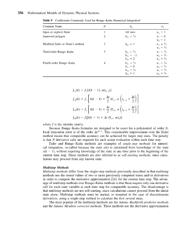
Table 9 Coefficients Commonly Used for Runge–Kutta Numerical Integration 6
Common Name N b jl w j
Open or explicit Euler 1 All zero w 1 1
1
Improved polygon 2 b 21 ⁄2 w 1 0
w 2 1
1
Modified Euler or Heun’s method 2 b 21 1 w 1 ⁄2
1
w 2 ⁄2
1
1
Third-order Runge–Kutta 3 b 21 ⁄2 w 1 ⁄6
2
b 31 1 w 2 ⁄3
1
b 32 2 w 3 ⁄6
1
1
Fourth-order Runge–Kutta 4 b 21 ⁄2 w 1 ⁄6
1
b 31 0 w 2 ⁄3
1 1
b 32 ⁄2 w 3 ⁄3
1
b 43 1 w 4 ⁄6
ƒ(k) ƒ[˜x(k 1), u(t k 1 )]
i
i1
ƒ(k) ƒ
˜ x(k 1) t Iƒ, ut
k 1
t
i1
i
i2
2
2
ƒ(k) ƒ
t
t
i2
i3 i ˜ x(k 1) Iƒ, ut
k 1
2 2
ƒ(k) ƒ[˜x(k 1) tIƒ, u(t )]
k
i
i4
i3
where I is the identity matrix.
Because Runge–Kutta formulas are designed to be exact for a polynomial of order N,
local truncation error is of the order t N 1 . This considerable improvement over the Euler
method means that comparable accuracy can be achieved for larger step sizes. The penalty
is that N derivative calls are required for each scalar evaluation within each time step.
Euler and Runge–Kutta methods are examples of single-step methods for numeri-
cal integration, so-called because the state x(k) is calculated from knowledge of the state
x(k 1), without requiring knowledge of the state at any time prior to the beginning of the
current time step. These methods are also referred to as self-starting methods, since calcu-
lations may proceed from any known state.
Multistep Methods
Multistep methods differ from the single-step methods previously described in that multistep
methods use the stored values of two or more previously computed states and/or derivatives
˜
in order to compute the derivative approximation ƒ (k) for the current time step. The advan-
i
tage of multistep methods over Runge–Kutta methods is that these require only one derivative
call for each state variable at each time step for comparable accuracy. The disadvantage is
that multistep methods are not self-starting, since calculations cannot proceed from the initial
state alone. Multistep methods must be started, or restarted in the case of discontinuous
derivatives, using a single-step method to calculate the first several steps.
The most popular of the multistep methods are the Adams–Bashforth predictor methods
and the Adams–Moulton corrector methods. These methods use the derivative approximation