
Page 369 - Mechanical Engineers' Handbook (Volume 2)
P. 369
360 Mathematical Models of Dynamic Physical Systems
3
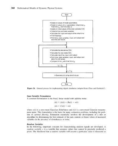
Figure 26 General process for implementing digital simulation (adapted from Close and Frederick ).
State-Variable Formulation
A common formulation is the fixed, linear model with additive noise
˙ x(t) Ax(t) Bu(t) w(t)
y(t) Cx(t) v(t)
where w(t) is a zero-mean Gaussian disturbance and v(t) is a zero-mean Gaussian measure-
ment noise. This formulation is the basis for many estimation problems, including the prob-
lem of optimal filtering. Estimation essentially involves the development of a rule or
algorithm for determining the best estimate of the past, current, or future values of measured
variables in the presence of disturbances or noise.
Random Variables
In the following, important concepts for characterizing random signals are developed. A
random variable x is a variable that assumes values that cannot be precisely predicted a
priori. The likelihood that a random variable will assume a particular value is measured as